Predictive modeling of reliability engineering data using a new version of the flexible Weibull model

Walid Emam; Ghadah Alomani; Walid Emam; Ghadah Alomani

doi:10.3934/mbe.2023436

Mathematical Biosciences and Engineering

2023, Volume 20, Issue 6: 9948-9964. doi: 10.3934/mbe.2023436

Previous Article Next Article

Research article Special Issues

Predictive modeling of reliability engineering data using a new version of the flexible Weibull model

Walid Emam ^{1
,
,},
Ghadah Alomani ²

1.
Department of Statistics and Operation Research, Faculty of Science, King Saud University, P.O.Box 2455, Riyadh 11451, Saudi Arabia
2.
Department of Mathematical Sciences, College of Science, Princess Nourah bint Abdulrahman University, P.O. Box 84428, Riyadh 11671, Saudi Arabia

Academic Editor: Xiaodi Li

Received: 11 December 2022 Revised: 04 February 2023 Accepted: 20 February 2023 Published: 27 March 2023

The combined-unified hybrid sampling approach was introduced as a general model that combines the unified hybrid censoring sampling approach and the combined hybrid censoring approach into a unified approach. In this paper, we apply this censoring sampling approach to improve the estimation of the parameter via a novel five-parameter expansion distribution, which we call the generalized Weibull-modified Weibull model. The new distribution contains five parameters and is therefore very flexible in terms of accommodating different types of data. The new distribution provides graphs of the probability density function, e.g., symmetric or right skewed. The graph of the risk function can have a shape similar to a monomer of the increasing or decreasing model. Using the Monte Carlo method, the maximum likelihood approach is used in the estimation procedure. The Copula model was used to discuss the two marginal univariate distributions. The asymptotic confidence intervals of the parameters were developed. We present some simulation results to validate the theoretical results. Finally, a data set with failure times for 50 electronic components was analyzed to illustrate the applicability and potential of the proposed model.
- modified Weibull,
- generalized Weibull,
- maximum likelihood estimation,
- statistical modeling
Citation: Walid Emam, Ghadah Alomani. Predictive modeling of reliability engineering data using a new version of the flexible Weibull model[J]. Mathematical Biosciences and Engineering, 2023, 20(6): 9948-9964. doi: 10.3934/mbe.2023436

Related Papers:

Abstract

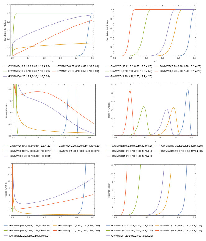
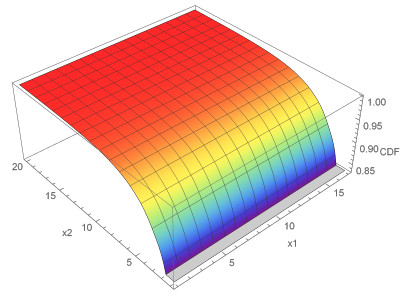
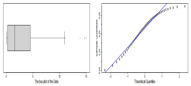
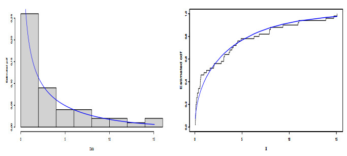
The combined-unified hybrid sampling approach was introduced as a general model that combines the unified hybrid censoring sampling approach and the combined hybrid censoring approach into a unified approach. In this paper, we apply this censoring sampling approach to improve the estimation of the parameter via a novel five-parameter expansion distribution, which we call the generalized Weibull-modified Weibull model. The new distribution contains five parameters and is therefore very flexible in terms of accommodating different types of data. The new distribution provides graphs of the probability density function, e.g., symmetric or right skewed. The graph of the risk function can have a shape similar to a monomer of the increasing or decreasing model. Using the Monte Carlo method, the maximum likelihood approach is used in the estimation procedure. The Copula model was used to discuss the two marginal univariate distributions. The asymptotic confidence intervals of the parameters were developed. We present some simulation results to validate the theoretical results. Finally, a data set with failure times for 50 electronic components was analyzed to illustrate the applicability and potential of the proposed model.

References

[1]	W. Emam, Y. Tashkandy, The Weibull claim model: Bivariate extension, Bayesian, and maximum likelihood estimations, Math. Probl. Eng., 2022 (2022), 1–10. https://doi.org/10.1155/2022/8729529 doi: 10.1155/2022/8729529
[2]	W. Emam, Y. Tashkandy, A new generalized modified Weibull model: Simulating and modeling the dynamics of the COVID-19 pandemic in Saudi Arabia and Egypt, Math. Probl. Eng., 2022 (2022), 1–9. https://doi.org/10.1155/2022/1947098 doi: 10.1155/2022/1947098
[3]	X. Liu, Z. Ahmad, S. K. Khosa, M. Yusuf, O. Alamri, W. Emam, A new flexible statistical model: Simulating and modeling the survival times of COVID-19 patients in China, Complexity, 2021 (2021), 1–16. https://doi.org/10.1155/2021/6915742 doi: 10.1155/2021/6915742
[4]	W. Emam, Y. Tashkandy, The arcsine Kumaraswamy-generalized family: Bayesian and classical estimates and application, Symmetry, 14 (2022), 2311. https://doi.org/10.3390/sym14112311 doi: 10.3390/sym14112311
[5]	W. Emam, Y. Tashkandy, Khalil new generalized Weibull distribution based on ranked samples: Estimation, mathematical properties, and application to COVID-19 data, Symmetry, 14 (2022), 853. https://doi.org/10.3390/sym14050853 doi: 10.3390/sym14050853
[6]	G. M. Cordeiro, E. M. M. Ortega, T. G. Ramires, A new generalized Weibull family of distributions: Mathematical properties and applications, J. Stat. Distrib. Appl., 2 (2015), 1–25. https://doi.org/10.1186/s40488-015-0036-6 doi: 10.1186/s40488-015-0036-6
[7]	B. Epstein, Truncated life tests in the exponential case, Ann. Math. Stat., 25 (1954), 555–564.
[8]	H. S. Jeong, J. I. Park, B. J. Yum, Development of $(r, T)$ hybrid sampling plans for exponential lifetime distributions, J. Appl. Stat., 23 (1996), 601–607. https://doi.org/10.1080/02664769623964 doi: 10.1080/02664769623964
[9]	A. Childs, B. Chandrasekhar, N. Balakrishnan, D. Kundu, Exact likelihood inference based on type-I and type-Ⅱ hybrid censored samples from the exponential distribution, Ann. Inst. Stat. Math., 55 (2003), 319–330. https://doi.org/10.1007/BF02530502 doi: 10.1007/BF02530502
[10]	X. P. Xiao, H. Guo, S. H. Mao, The modeling mechanism, extension and optimization of grey GM (1, 1) model, Appl. Math. Modell., 38 (2014), 1896–1910. https://doi.org/10.1016/j.apm.2013.10.004 doi: 10.1016/j.apm.2013.10.004
[11]	N. Balakrishnan, D. Kundu, Hybrid censoring: Models, inferential results and applications, Comput. Stat. Data Anal., 57 (2013), 166–209. https://doi.org/10.1016/j.csda.2012.03.025 doi: 10.1016/j.csda.2012.03.025
[12]	S. Chen, G. K. Bhattacharya, Exact confidence bounds for an exponential parameter under hybrid censoring, Commun. Stat. Theory Methods, 16 (1987), 2429–2442. https://doi.org/10.1080/03610928708829516 doi: 10.1080/03610928708829516
[13]	N. Draper, I. Guttman, Bayesian analysis of hybrid life tests with exponential failure times, Ann. Inst. Stat. Math., 39 (1987), 219–225. https://doi.org/10.1007/BF02491461 doi: 10.1007/BF02491461
[14]	K. Fairbanks, R. Madson, R. Dykstra, A confidence interval for an exponential parameter from a hybrid life test, J. Am. Stat. Assoc., 77 (1982), 137–140.
[15]	N. Balakrishnan, A. Rasouli, N. S. Farsipour, Exact likelihood inference based on an unified hybrid censored sample from the exponential distribution. J. Stat. Comput. Simul., 78 (2008), 475–488. https://doi.org/10.1080/00949650601158336 doi: 10.1080/00949650601158336
[16]	W. T. Huang, K. C. Yang, A new hybrid censoring scheme and some of its properties, Tamsui Oxford J. Math. Sci., 26 (2010), 355–367.
[17]	W. Emam, K. S. Sultan, Bayesian and maximum likelihood estimations of the Dagum parameters under combined-unified hybrid censoring, Math. Biosci. Eng., 18 (2021), 2930–2951. http://dx.doi.org/10.3934/mbe.2021148 doi: 10.3934/mbe.2021148
[18]	A. M. Sarhan, M. Zaindin, Modified Weibull distribution, APPS Appl. Sci., 11 (2009), 123–136.
[19]	D. Morgenstern, Einfache beispiele zweidimensionaler verteilungen, Mitt. Math. Statist., 8 (1956), 234–235.
[20]	D. A. Conway, Farlie-Gumbel-Morgenstern distributions, in Encyclopedia of Statistical Sciences, (eds. Kotz and N. L. Johnson), Wiley, (1983), 28–31.
[21]	A. Xu, S. Zhou, Y. Tang, A unified model for system reliability evaluation under dynamic operating conditions, IEEE Trans. Reliab., 70 (2019), 65–72. https://doi.org/10.1109/TR.2019.2948173 doi: 10.1109/TR.2019.2948173
[22]	C. Luo, L. Shen, A. Xu, Modelling and estimation of system reliability under dynamic operating environments and lifetime ordering constraints, Reliab. Eng. Syst. Saf., 218 (2022), 108136. https://doi.org/10.1016/j.ress.2021.108136 doi: 10.1016/j.ress.2021.108136
[23]	G. Aryal, I. Elbatal, On the exponentiated generalized modified Weibull distribution, Commun. Stat. Appl. Methods, 22 (2015), 333–348. http://dx.doi.org/10.5351/CSAM.2015.22.4.333 doi: 10.5351/CSAM.2015.22.4.333
[24]	L. Zhang, A. Xu, L. An, M. Li, Bayesian inference of system reliability for multicomponent stress-strength model under Marshall-Olkin Weibull distribution, Systems, 10 (2022), 196. https://doi.org/10.3390/systems10060196 doi: 10.3390/systems10060196
[25]	L. Zhuang, A. Xu, B. Wang, Y. Xue, S. Zhang, Data analysis of progressive-stress accelerated life tests with group effects, Qual. Technol. Quant. Manage., 2022 (2022), 1–21. https://doi.org/10.1080/16843703.2022.2147690 doi: 10.1080/16843703.2022.2147690

Reader Comments

Your name:*

Email:*
© 2023 the Author(s), licensee AIMS Press. This is an open access article distributed under the terms of the Creative Commons Attribution License (http://creativecommons.org/licenses/by/4.0)