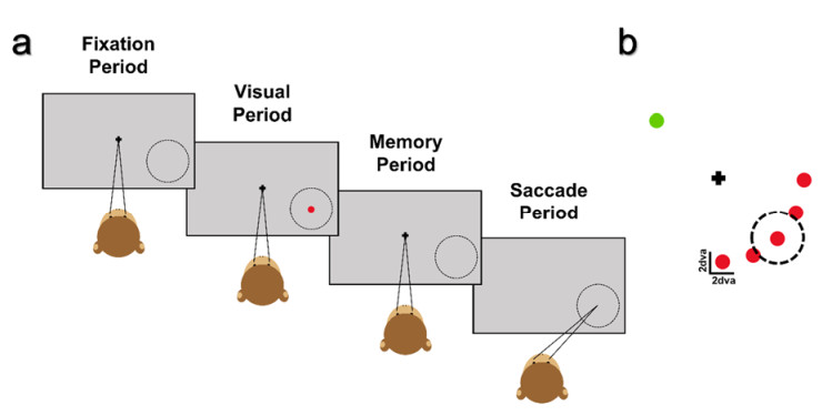
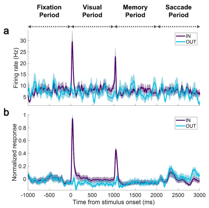
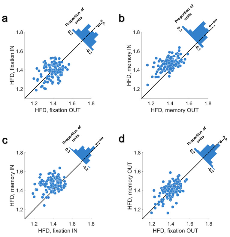
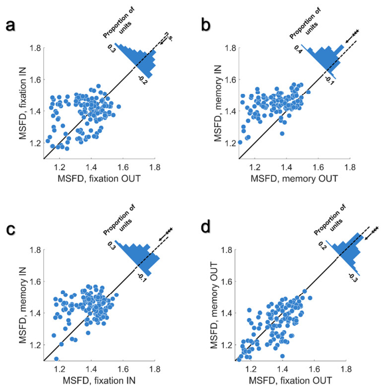
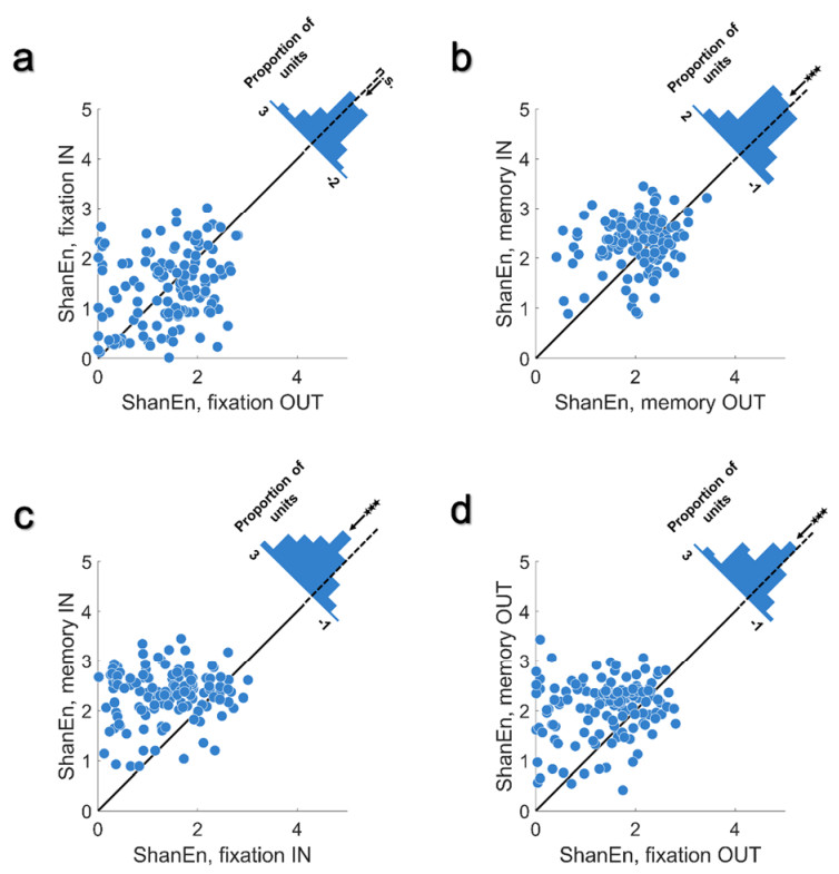
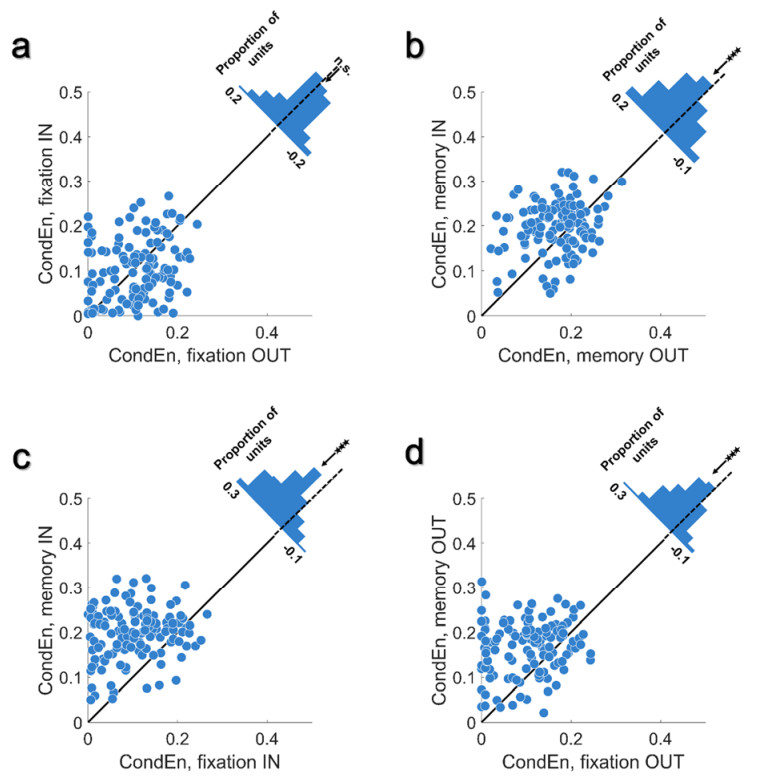
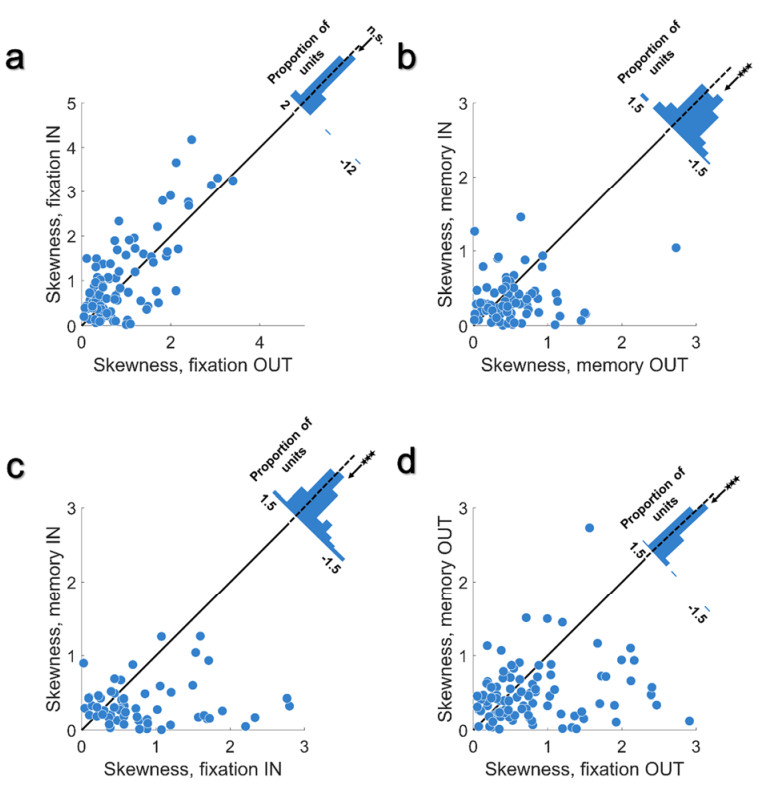
Working memory has been identified as a top-down modulation of the average spiking activity in different brain parts. However, such modification has not yet been reported in the middle temporal (MT) cortex. A recent study showed that the dimensionality of the spiking activity of MT neurons increases after deployment of spatial working memory. This study is devoted to analyzing the ability of nonlinear and classical features to capture the content of the working memory from the spiking activity of MT neurons. The results suggest that only the Higuchi fractal dimension can be considered as a unique indicator of working memory while the Margaos-Sun fractal dimension, Shannon entropy, corrected conditional entropy, and skewness are perhaps indicators of other cognitive factors such as vigilance, awareness, and arousal as well as working memory.
Citation: Gayathri Vivekanandhan, Mahtab Mehrabbeik, Karthikeyan Rajagopal, Sajad Jafari, Stephen G. Lomber, Yaser Merrikhi. Higuchi fractal dimension is a unique indicator of working memory content represented in spiking activity of visual neurons in extrastriate cortex[J]. Mathematical Biosciences and Engineering, 2023, 20(2): 3749-3767. doi: 10.3934/mbe.2023176
Working memory has been identified as a top-down modulation of the average spiking activity in different brain parts. However, such modification has not yet been reported in the middle temporal (MT) cortex. A recent study showed that the dimensionality of the spiking activity of MT neurons increases after deployment of spatial working memory. This study is devoted to analyzing the ability of nonlinear and classical features to capture the content of the working memory from the spiking activity of MT neurons. The results suggest that only the Higuchi fractal dimension can be considered as a unique indicator of working memory while the Margaos-Sun fractal dimension, Shannon entropy, corrected conditional entropy, and skewness are perhaps indicators of other cognitive factors such as vigilance, awareness, and arousal as well as working memory.

| [1] |
E. K. Miller, M. Lundqvist, A. M. Bastos, Working memory 2.0, Neuron, 100 (2018), 463–475. https://doi.org/10.1016/j.neuron.2018.09.023 doi: 10.1016/j.neuron.2018.09.023

|
| [2] |
A. Baddeley, Working memory, Science, 255 (1992), 556–559. https://doi.org/10.1126/science.1736359 doi: 10.1126/science.1736359
|
| [3] |
A. Baddeley, Working memory and language: An overview, J. Commun. Disord., 36 (2003), 189–208. https://doi.org/10.1016/S0021-9924(03)00019-4 doi: 10.1016/S0021-9924(03)00019-4
|
| [4] |
Y. Merrikhi, M. Shams-Ahmar, H. Karimi-Rouzbahani, K. Clark, R. Ebrahimpour, B. Noudoost, Dissociable contribution of extrastriate responses to representational enhancement of gaze targets, J. Cognit. Neurosci., 33 (2021), 2167–2180. https://doi.org/10.1162/jocn_a_01750 doi: 10.1162/jocn_a_01750
|
| [5] |
R. M. Alderson, L. J. Kasper, K. L. Hudec, C. H. G. Patros, Attention-deficit/hyperactivity disorder (ADHD) and working memory in adults: a meta-analytic review, Neuropsychology, 27 (2013), 287. https://doi.org/10.1037/a0032371 doi: 10.1037/a0032371
|
| [6] |
S. J. Luck, J. M. Gold, The construct of attention in schizophrenia, Biol. Psychiatry, 64 (2008), 34–39. https://doi.org/10.1016/j.biopsych.2008.02.014 doi: 10.1016/j.biopsych.2008.02.014
|
| [7] |
E. Awh, J. Jonides, Overlapping mechanisms of attention and spatial working memory, Trends Cognit. Sci., 5 (2001), 119–126. https://doi.org/10.1016/S1364-6613(00)01593-X doi: 10.1016/S1364-6613(00)01593-X
|
| [8] |
Y. Merrikhi, K. Clark, E. Albarran, M. Parsa, M. Zirnsak, T. Moore, et al., Spatial working memory alters the efficacy of input to visual cortex, Nat. Commun., 8 (2017), 15041. https://doi.org/10.1038/ncomms15041 doi: 10.1038/ncomms15041
|
| [9] |
D. Mendoza-Halliday, S. Torres, J. C. Martinez-Trujillo, Sharp emergence of feature-selective sustained activity along the dorsal visual pathway, Nat. Neurosci., 17 (2014), 1255–1262. https://doi.org/10.1038/nn.3785 doi: 10.1038/nn.3785
|
| [10] |
Y. Merrikhi, K. Clark, B. Noudoost, Concurrent influence of top-down and bottom-up inputs on correlated activity of Macaque extrastriate neurons, Nat. Commun., 9 (2018), 5393. https://doi.org/10.1038/s41467-018-07816-4 doi: 10.1038/s41467-018-07816-4
|
| [11] |
S. Kastner, K. DeSimone, C. S. Konen, S. M. Szczepanski, K. S. Weiner, K. A. Schneider, Topographic maps in human frontal cortex revealed in memory-guided saccade and spatial working-memory tasks, J. Neurophysiol., 97 (2007), 3494–3507. https://doi.org/10.1152/jn.00010.2007 doi: 10.1152/jn.00010.2007
|
| [12] |
A. Charef, H. Sun, Y. Tsao, B. Onaral, Fractal system as represented by singularity function, IEEE Trans. Autom. Control, 37 (1992), 1465–1470. https://doi.org/10.1109/9.159595 doi: 10.1109/9.159595
|
| [13] |
B. Y. Hayden, J. L. Gallant, Working memory and decision processes in visual area v4, Front. Neurosci., 7 (2013), 18. https://doi.org/10.3389/fnins.2013.00018 doi: 10.3389/fnins.2013.00018
|
| [14] |
M. L. Leavitt, D. Mendoza-Halliday, J. C. Martinez-Trujillo, Sustained activity encoding working memories: not fully distributed, Trends Neurosci., 40 (2017), 328–346. https://doi.org/10.1016/j.tins.2017.04.004 doi: 10.1016/j.tins.2017.04.004
|
| [15] |
J. Spilka, V. Chudáček, M. Koucký, L. Lhotská, M. Huptych, P. Janků, et al., Using nonlinear features for fetal heart rate classification, Biomed. Signal Process. Control, 7 (2012), 350–357. https://doi.org/10.1016/j.bspc.2011.06.008 doi: 10.1016/j.bspc.2011.06.008
|
| [16] |
H. Namazi, R. Khosrowabadi, J. Hussaini, S. Habibi, A. A. Farid, V. V. Kulish, Analysis of the influence of memory content of auditory stimuli on the memory content of EEG signal, Oncotarget, 7 (2016), 56120. https://doi.org/10.18632/oncotarget.11234 doi: 10.18632/oncotarget.11234
|
| [17] |
V. Jahmunah, S. L. Oh, V. Rajinikanth, E. J. Ciaccio, K. H. Cheong, N. Arunkumar, et al., Automated detection of schizophrenia using nonlinear signal processing methods, Artif. Intell. Med., 100 (2019), 101698. https://doi.org/10.1016/j.artmed.2019.07.006 doi: 10.1016/j.artmed.2019.07.006
|
| [18] |
H. Namazi, O. Krejcar, Analysis of pregnancy development by complexity and information-based analysis of fetal phonocardiogram (PCG) signals, Fluct. Noise Lett., 20 (2021), 2150028. https://doi.org/10.1142/S0219477521500280 doi: 10.1142/S0219477521500280
|
| [19] |
M. Mehrabbeik, M. Shams-Ahmar, A. T. Levine, S. Jafari, Y. Merrikhi, Distinctive nonlinear dimensionality of neural spiking activity in extrastriate cortex during spatial working memory; a Higuchi fractal analysis, Chaos, Solitons Fractals, 158 (2022), 112051. https://doi.org/10.1016/j.chaos.2022.112051 doi: 10.1016/j.chaos.2022.112051
|
| [20] |
H. Namazi, Can we mathematically correlate brain memory and complexity, ARC J. Neurosci., 3 (2018), 10–12. https://doi.org/10.20431/2456-057X.0302003 doi: 10.20431/2456-057X.0302003
|
| [21] |
H. Namazi, M. R. Ashfaq Ahamed, M. H. Babini, O. Krejcar, Analysis of the correlation between the human voice and brain activity, Waves Random Complex Media, 2021 (2021), 1–13. https://doi.org/10.1080/17455030.2021.1921313 doi: 10.1080/17455030.2021.1921313
|
| [22] |
T. Higuchi, Approach to an irregular time series on the basis of the fractal theory, Physica D, 31 (1988), 277–283. https://doi.org/10.1016/0167-2789(88)90081-4 doi: 10.1016/0167-2789(88)90081-4
|
| [23] |
M. J. Katz, Fractals and the analysis of waveforms, Comput. Biol. Med., 18 (1988), 145–156. https://doi.org/10.1016/0010-4825(88)90041-8 doi: 10.1016/0010-4825(88)90041-8
|
| [24] |
T. Di Matteo, Multi-scaling in finance, Quant. Finance, 7 (2007), 21–36. https://doi.org/10.1080/14697680600969727 doi: 10.1080/14697680600969727
|
| [25] |
P. Maragos, F. Sun, Measuring the fractal dimension of signals: Morphological covers and iterative optimization, IEEE Trans. Signal Process., 41 (1993), 108. https://doi.org/10.1109/TSP.1993.193131 doi: 10.1109/TSP.1993.193131
|
| [26] |
L. S. Liebovitch, T. Toth, A fast algorithm to determine fractal dimensions by box counting, Phys. Lett. A, 141 (1989), 386–390. https://doi.org/10.1016/0375-9601(89)90854-2 doi: 10.1016/0375-9601(89)90854-2
|
| [27] |
K. Suganthi, G. Jayalalitha, Geometric Brownian Motion in Stock prices, J. Phys. Conf. Ser., 1377 (2019), 012016. https://doi.org/10.1088/1742-6596/1377/1/012016 doi: 10.1088/1742-6596/1377/1/012016
|
| [28] |
A. Delgado-Bonal, A. Marshak, Approximate entropy and sample entropy: A comprehensive tutorial, Entropy, 21 (2019). https://doi.org/10.3390/e21060541 doi: 10.3390/e21060541
|
| [29] |
J. S. Richman, J. R. Moorman, Physiological time-series analysis using approximate entropy and sample entropy, Am. J. Physiol. Heart Circ. Physiol., 278 (2000), H2039–H2049. https://doi.org/10.1152/ajpheart.2000.278.6.H2039 doi: 10.1152/ajpheart.2000.278.6.H2039
|
| [30] |
A. Porta, G. Baselli, D. Liberati, N. Montano, C. Cogliati, T. Gnecchi-Ruscone, et al., Measuring regularity by means of a corrected conditional entropy in sympathetic outflow, Biol. Cybern., 78 (1998), 71–78. https://doi.org/10.1007/s004220050414 doi: 10.1007/s004220050414
|
| [31] |
C. Bandt, B. Pompe, Permutation entropy: A natural complexity measure for time series, Phys. Rev. Lett., 88 (2002), 174102. https://doi.org/10.1103/PhysRevLett.88.174102 doi: 10.1103/PhysRevLett.88.174102
|
| [32] |
W. Chen, Z. Wang, H. Xie, W. Yu, Characterization of surface EMG signal based on fuzzy entropy, IEEE Trans. Neural Syst. Rehabil. Eng., 15 (2007), 266–272. https://doi.org/10.1109/TNSRE.2007.897025 doi: 10.1109/TNSRE.2007.897025
|
| [33] |
Z. Gao, W. Dang, X. Wang, X. Hong, L. Hou, K. Ma, et al., Complex networks and deep learning for EEG signal analysis, Cognit. Neurodyn., 15 (2021), 369–388. https://doi.org/10.1007/s11571-020-09626-1 doi: 10.1007/s11571-020-09626-1
|
| [34] |
R. K. Guntu, P. K. Yeditha, M. Rathinasamy, M. Perc, N. Marwan, J. Kurths, et al., Wavelet entropy-based evaluation of intrinsic predictability of time series, Chaos, 30 (2020), 033117. https://doi.org/10.1063/1.5145005 doi: 10.1063/1.5145005
|
| [35] | D. Zhang, Wavelet transform, in Fundamentals of Image Data Mining: Analysis, Features, Classification and Retrieval, Springer International Publishing, (2019). 35–44. https://doi.org/10.1007/978-3-030-17989-2_3 |
| [36] | R. M. Rangayyan, Biomedical Signal Analysis, John Wiley & Sons, 2015. https://doi.org/10.1002/9781119068129 |
| [37] |
H. H. Giv, Directional short-time Fourier transform, J. Math. Anal. Appl., 399 (2013), 100–107. https://doi.org/10.1016/j.jmaa.2012.09.053 doi: 10.1016/j.jmaa.2012.09.053
|
| [38] |
N. Ahmed, T. Natarajan, K. R. Rao, Discrete cosine transform, IEEE Trans. Comput., 100 (1974), 90–93. https://doi.org/10.1109/T-C.1974.223784 doi: 10.1109/T-C.1974.223784
|
| [39] | M. Feldman, Hilbert transforms, in Encyclopedia of Vibration, Elsevier, (2001), 642–648. https://doi.org/10.1006/rwvb.2001.0057 |
| [40] |
R. G. Stockwell, L. Mansinha, R. P. Lowe, Localization of the complex spectrum: the S transform, IEEE Trans. Signal Process., 44 (1996), 998–1001. https://doi.org/10.1109/78.492555 doi: 10.1109/78.492555
|
Figures(7) / Tables(8)

Gayathri Vivekanandhan, Mahtab Mehrabbeik, Karthikeyan Rajagopal, Sajad Jafari, Stephen G. Lomber, Yaser Merrikhi. Higuchi fractal dimension is a unique indicator of working memory content represented in spiking activity of visual neurons in extrastriate cortex[J]. Mathematical Biosciences and Engineering, 2023, 20(2): 3749-3767. doi: 10.3934/mbe.2023176


 DownLoad: