An efficient coverage method for SEMWSNs based on adaptive chaotic Gaussian variant snake optimization algorithm

Xiang Liu; Min Tian; Jie Zhou; Jinyan Liang; Xiang Liu; Min Tian; Jie Zhou; Jinyan Liang

doi:10.3934/mbe.2023150

Mathematical Biosciences and Engineering

2023, Volume 20, Issue 2: 3191-3215. doi: 10.3934/mbe.2023150

Previous Article Next Article

Research article Special Issues

An efficient coverage method for SEMWSNs based on adaptive chaotic Gaussian variant snake optimization algorithm

1.
College of mechanical and electrical engineering, Shihezi University, Shihezi 832000, China
2.
College of information science and technology, Shihezi University, Shihezi 832000, China

Academic Editor: Wenqiang Zhang

Received: 08 October 2022 Revised: 21 November 2022 Accepted: 25 November 2022 Published: 02 December 2022

Soil element monitoring wireless sensor networks (SEMWSNs) are widely used in soil element monitoring agricultural activities. SEMWSNs monitor changes in soil elemental content during agriculture products growing through nodes. Based on the feedback from the nodes, farmers adjust irrigation and fertilization strategies on time, thus promoting the economic growth of crops. The critical issue in SEMWSNs coverage studies is to achieve maximum coverage of the entire monitoring field by adopting a smaller number of sensor nodes. In this study, a unique adaptive chaotic Gaussian variant snake optimization algorithm (ACGSOA) is proposed for solving the above problem, which also has the advantages of solid robustness, low algorithmic complexity, and fast convergence. A new chaotic operator is proposed in this paper to optimize the position parameters of individuals, enhancing the convergence speed of the algorithm. Moreover, an adaptive Gaussian variant operator is also designed in this paper to effectively avoid SEMWSNs from falling into local optima during the deployment process. Simulation experiments are designed to compare ACGSOA with other widely used metaheuristics, namely snake optimizer (SO), whale optimization algorithm (WOA), artificial bee colony algorithm (ABC), and fruit fly optimization algorithm (FOA). The simulation results show that the performance of ACGSOA has been dramatically improved. On the one hand, ACGSOA outperforms other methods in terms of convergence speed, and on the other hand, the coverage rate is improved by 7.20%, 7.32%, 7.96%, and 11.03% compared with SO, WOA, ABC, and FOA, respectively.
- coverage optimization,
- snake optimizer,
- chaotic operator,
- Gaussian variant,
- power consumption
Citation: Xiang Liu, Min Tian, Jie Zhou, Jinyan Liang. An efficient coverage method for SEMWSNs based on adaptive chaotic Gaussian variant snake optimization algorithm[J]. Mathematical Biosciences and Engineering, 2023, 20(2): 3191-3215. doi: 10.3934/mbe.2023150

Related Papers:

Abstract

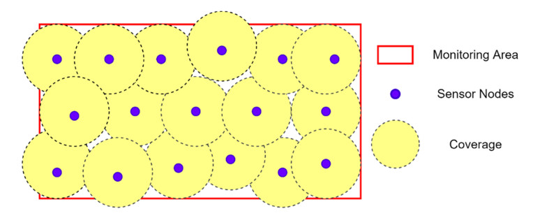
Soil element monitoring wireless sensor networks (SEMWSNs) are widely used in soil element monitoring agricultural activities. SEMWSNs monitor changes in soil elemental content during agriculture products growing through nodes. Based on the feedback from the nodes, farmers adjust irrigation and fertilization strategies on time, thus promoting the economic growth of crops. The critical issue in SEMWSNs coverage studies is to achieve maximum coverage of the entire monitoring field by adopting a smaller number of sensor nodes. In this study, a unique adaptive chaotic Gaussian variant snake optimization algorithm (ACGSOA) is proposed for solving the above problem, which also has the advantages of solid robustness, low algorithmic complexity, and fast convergence. A new chaotic operator is proposed in this paper to optimize the position parameters of individuals, enhancing the convergence speed of the algorithm. Moreover, an adaptive Gaussian variant operator is also designed in this paper to effectively avoid SEMWSNs from falling into local optima during the deployment process. Simulation experiments are designed to compare ACGSOA with other widely used metaheuristics, namely snake optimizer (SO), whale optimization algorithm (WOA), artificial bee colony algorithm (ABC), and fruit fly optimization algorithm (FOA). The simulation results show that the performance of ACGSOA has been dramatically improved. On the one hand, ACGSOA outperforms other methods in terms of convergence speed, and on the other hand, the coverage rate is improved by 7.20%, 7.32%, 7.96%, and 11.03% compared with SO, WOA, ABC, and FOA, respectively.

References

[1]	A. Rejeb, K. Rejeb, A. Abdollahi, F. Al-Turjman, H. Treiblmaier, The Interplay between the Internet of Things and agriculture: A bibliometric analysis and research agenda, Internet Things, 19 (2022), 100580. https://doi.org/10.1016/j.iot.2022.100580 doi: 10.1016/j.iot.2022.100580
[2]	T. Ojha, S. Misra, N. S. Raghuwanshi, Wireless sensor networks for agriculture: The state-of-the-art in practice and future challenges, Comput. Electron. Agric., 118 (2015), 66–84. https://doi.org/10.1016/j.compag.2015.08.011 doi: 10.1016/j.compag.2015.08.011
[3]	S. M. Mohamed, H. S. Hamza, I. A. Saroit, Coverage in mobile wireless sensor networks (M-WSN): A survey, Comput. Commun., 110 (2017), 133–150. https://doi.org/10.1016/j.comcom.2017.06.010 doi: 10.1016/j.comcom.2017.06.010
[4]	J. Zhou, Y. Zhang, Z. Li, R. Zhu, A. zeman, Stochastic scheduling of a power grid in the presence of EVs, RESs, and risk index with a developed lightning search algorithm, J. Cleaner Prod., 364 (2022), 132473. https://doi.org/10.1016/j.jclepro.2022.132473 doi: 10.1016/j.jclepro.2022.132473
[5]	M. K. B. Melhem, L. Abualigah, R. A. Zitar, A. G. Hussien, D. Oliva, Comparative study on arabic text classification: challenges and opportunities, in Classification Applications with Deep Learning and Machine Learning Technologies, Springer, Cham, (2023), 217–224. https://doi.org/10.1007/978-3-031-17576-3_10
[6]	N. Milhem, L. Abualigah, M. H. Nadimi-Shahraki, H. Jia, A. E. Ezugwu, A. G. Hussien, Enhanced MapReduce performance for the distributed parallel computing: application of the big data, in Classification Applications with Deep Learning and Machine Learning Technologies, Springer, Cham, (2023), 191–203. https://doi.org/10.1007/978-3-031-17576-3_8
[7]	C. Li, Y. Liu, Y. Zhang, M. Xu, J. Xiao, J. Zhou, A novel nature-inspired routing scheme for improving routing quality of service in power grid monitoring systems, IEEE Syst. J., 2022 (2022), 1–12. https://doi.org/10.1109/jsyst.2022.3192856 doi: 10.1109/jsyst.2022.3192856
[8]	L. Cao, Y. Yue, Y. Cai, Y. Zhang, A novel coverage optimization strategy for heterogeneous wireless sensor networks based on connectivity and reliability, IEEE Access, 9 (2021), 18424–18442. https://doi.org/10.1109/access.2021.3053594 doi: 10.1109/access.2021.3053594
[9]	J. Lloret, S. Sendra, L. Garcia, J. M. Jimenez, A wireless sensor network deployment for soil moisture monitoring in precision agriculture, Sensors, 21 (2021), 7243. https://doi.org/10.3390/s21217243 doi: 10.3390/s21217243
[10]	J. Amutha, S. Sharma, J. Nagar, WSN strategies based on sensors, deployment, sensing models, coverage and energy efficiency: review, approaches and open issues, Wireless Pers. Commun., 111 (2020), 1089–1115. https://doi.org/10.1007/s11277-019-06903-z doi: 10.1007/s11277-019-06903-z
[11]	S. Q. Ong, G. Nair, R. D. A. Dabbagh, N. F. Aminuddin, P. Sumari, L. Abualigah, et al., Comparison of pre-trained and convolutional neural networks for classification of jackfruit artocarpus integer and artocarpus heterophyllus, in Classification Applications with Deep Learning and Machine Learning Technologies, Springer, Cham, (2023), 129–141. https://doi.org/10.1007/978-3-031-17576-3_6
[12]	S. Verma, N. Sood, A. K. Sharma, Genetic algorithm-based optimized cluster head selection for single and multiple data sinks in heterogeneous wireless sensor network, Appl. Soft Comput., 85 (2019), 105788. https://doi.org/10.1016/j.asoc.2019.105788 doi: 10.1016/j.asoc.2019.105788
[13]	R. Priyadarshi, P. Rawat, V. Nath, Energy dependent cluster formation in heterogeneous wireless sensor network, Microsyst. Technol., 25 (2019), 2313–2321. https://doi.org/10.1007/s00542-018-4116-7 doi: 10.1007/s00542-018-4116-7
[14]	R. Moazenzadeh, B. Mohammadi, Assessment of bio-inspired metaheuristic optimisation algorithms for estimating soil temperature, Geoderma, 353(2019), 152–171. https://doi.org/10.1016/j.geoderma.2019.06.028 doi: 10.1016/j.geoderma.2019.06.028
[15]	Y. Liu, C. Li, Y. Zhang, M. Xu, J. Xiao, J. Zhou, HPCP-QCWOA: High performance clustering protocol based on quantum clone whale optimization algorithm in integrated energy system, Future Gener. Comput. Syst., 135 (2022), 315–332. https://doi.org/10.1016/j.future.2022.05.001 doi: 10.1016/j.future.2022.05.001
[16]	M. R. Tanweer, S. Suresh, N. Sundararajan, Self regulating particle swarm optimization algorithm, Inf. Sci., 294 (2015), 182–202. https://doi.org/10.1016/j.ins.2014.09.053 doi: 10.1016/j.ins.2014.09.053
[17]	C. Blum, Ant colony optimization: Introduction and recent trends, Phys. Life Rev., 2 (2005), 353–373. https://doi.org/10.1016/j.plrev.2005.10.001 doi: 10.1016/j.plrev.2005.10.001
[18]	A. A. Heidari, S. Mirjalili, H. Faris, I. Aljarah, M. Mafarja, H. Chen, Harris hawks optimization: Algorithm and applications, Future Gener. Comput. Syst., 97(2019), 849–872. https://doi.org/10.1016/j.future.2019.02.028 doi: 10.1016/j.future.2019.02.028
[19]	Y. Yang, H. Chen, A. A. Heidari, A. H. Gandomi, Hunger games search: Visions, conception, implementation, deep analysis, perspectives, and towards performance shifts, Expert Syst. Appl., 177 (2021), 114864. https://doi.org/10.1016/j.eswa.2021.114864 doi: 10.1016/j.eswa.2021.114864
[20]	G. G. Wang, S. Deb, Z. Cui, Monarch butterfly optimization, Neural Comput. Appl., 31 (2015), 1995–2014. https://doi.org/10.1007/s00521-015-1923-y doi: 10.1007/s00521-015-1923-y
[21]	R. Zheng, A. G. Hussien, H. M. Jia, L. Abualigah, S. Wang, D. Wu, An improved wild horse optimizer for solving optimization problems, Mathematics, 10 (2022), 1311. https://doi.org/10.3390/math10081311 doi: 10.3390/math10081311
[22]	R. Priyadarshi, B. Gupta, A. Anurag, Wireless sensor networks deployment: a result oriented analysis, Wireless Pers. Commun., 113 (2020), 843–866. https://doi.org/10.1007/s11277-020-07255-9 doi: 10.1007/s11277-020-07255-9
[23]	J. Liang, M. Tian, Y. Liu, J. Zhou, Coverage optimization of soil moisture wireless sensor networks based on adaptive Cauchy variant butterfly optimization algorithm, Sci. Rep., 12 (2022), 1–17. https://doi.org/10.1038/s41598-022-15689-3 doi: 10.1038/s41598-022-15689-3
[24]	H. Mostafaei, M. U. Chowdhury, M. S. Obaidat, Border surveillance With WSN systems in a distributed manner, IEEE Syst. J., 12 (2018), 3703–3712. https://doi.org/10.1109/jsyst.2018.2794583 doi: 10.1109/jsyst.2018.2794583
[25]	S. Saha, R. K. Arya, Adaptive virtual anchor node based underwater localization using improved shortest path algorithm and particle swarm optimization (PSO) technique, Concurrency Comput. Pract. Experi., 34 (2021), e6552. https://doi.org/10.1002/cpe.6552 doi: 10.1002/cpe.6552
[26]	N. T. Hanh, H. T. T. Binh, N. X. Hoai, M. S. Palaniswami, An efficient genetic algorithm for maximizing area coverage in wireless sensor networks, Inf. Sci., 488 (2019), 58–75. https://doi.org/10.1016/j.ins.2019.02.059 doi: 10.1016/j.ins.2019.02.059
[27]	J. W. Lee, J. J. Lee, Ant-colony-based scheduling algorithm for energy-efficient coverage of WSN, IEEE Sens. J., 12 (2012), 3036–3046. https://doi.org/10.1109/jsen.2012.2208742 doi: 10.1109/jsen.2012.2208742
[28]	A. G. Hussien, L. Abualigah, R. Abu Zitar, F. A. Hashim, M. Amin, A. Saber, et al., Recent advances in harris hawks optimization: A comparative study and applications, Electronics, 11 (2022), 1919. https://doi.org/10.3390/electronics11121919 doi: 10.3390/electronics11121919
[29]	A. G. Hussien, M. Amin, A self-adaptive Harris Hawks optimization algorithm with opposition-based learning and chaotic local search strategy for global optimization and feature selection, Int. J. Mach. Learn. Cybern., 13 (2022), 309–336. https://doi.org/10.1007/s13042-021-01326-4 doi: 10.1007/s13042-021-01326-4
[30]	R. Sharma, S. Prakash, HHO-LPWSN: harris hawks optimization algorithm for sensor nodes localization problem in wireless sensor networks, EAI Endorsed Trans. Scalable Inf. Syst., 8 (2018), e5. https://doi.org/10.4108/eai.25-2-2021.168807 doi: 10.4108/eai.25-2-2021.168807
[31]	A. G. Hussien, A. A. Heidari, X. Ye, G. Liang, H. Chen, Z. Pan, Boosting whale optimization with evolution strategy and Gaussian random walks: an image segmentation method, Eng. Comput., 2022 (2022), 1–45. https://doi.org/10.1007/s00366-021-01542-0 doi: 10.1007/s00366-021-01542-0
[32]	G. I. Sayed, G. Khoriba, M. H. Haggag, A novel chaotic salp swarm algorithm for global optimization and feature selection, Appl. Intell., 48 (2018), 3462–3481. https://doi.org/10.1007/s10489-018-1158-6 doi: 10.1007/s10489-018-1158-6
[33]	R. R. Mostafa, A. G. Hussien, M. A. Khan, S. Kadry, F. A. Hashim, Enhanced coot optimization algorithm for Dimensionality Reduction, in 2022 Fifth International Conference of Women in Data Science at Prince Sultan University (WiDS PSU), IEEE, Riyadh, Saudi Arabia, (2022), 43–48. https://doi.org/10.1109/WiDS-PSU54548.2022.00020
[34]	S. Wang, A. G. Hussien, H. Jia, L. Abualigah, R. Zheng, Enhanced remora optimization algorithm for solving constrained engineering optimization problems, Mathematics, 10 (2022), 1696. https://doi.org/10.3390/math10101696 doi: 10.3390/math10101696
[35]	A. G. Hussien, F. A. Hashim, R. Qaddoura, L. Abualigah, A. Pop, An enhanced evaporation rate water-cycle algorithm for global optimization, Processes, 10 (2022), 2254. https://doi.org/10.3390/pr10112254 doi: 10.3390/pr10112254
[36]	H. Yu, H. Jia, J. Zhou, A. G. Hussien, Enhanced Aquila optimizer algorithm for global optimization and constrained engineering problems, Math. Biosci. Eng., 19 (2022), 14173–14211. https://doi.org/10.3934/mbe.2022660 doi: 10.3934/mbe.2022660
[37]	I. Strumberger, M. Tuba, N. Bacanin, E. Tuba, Cloudlet scheduling by hybridized monarch butterfly optimization algorithm, J. Sens. Actuator Networks, 8(2019), 44. https://doi.org/10.3390/jsan8030044 doi: 10.3390/jsan8030044
[38]	I. Strumberger, E. Tuba, N. Bacanin, M. Beko, M. Tuba, Wireless sensor network localization problem by hybridized moth search algorithm, in 2018 14th International Wireless Communications & Mobile Computing Conference (IWCMC), IEEE, Limassol, Cyprus, (2018), 316–321. https://doi.org/10.1109/IWCMC.2018.8450491
[39]	F. K. Onay, S. B. Aydemı̇r, Chaotic hunger games search optimization algorithm for global optimization and engineering problems, Math. Comput. Simul., 192(2022), 514–536. https://doi.org/10.1016/j.matcom.2021.09.014 doi: 10.1016/j.matcom.2021.09.014
[40]	J. Daniel, S. F. V. Francis, S. Velliangiri, Cluster head selection in wireless sensor network using tunicate swarm butterfly optimization algorithm, Wireless Networks, 27 (2021), 5245–5262. https://doi.org/10.1007/s11276-021-02812-x doi: 10.1007/s11276-021-02812-x
[41]	R. Deepa, R. Venkataraman, Enhancing Whale Optimization Algorithm with Levy Flight for coverage optimization in wireless sensor networks, Comput. Electr. Eng., 94 (2021), 107359. https://doi.org/10.1016/j.compeleceng.2021.107359 doi: 10.1016/j.compeleceng.2021.107359
[42]	F. A. Hashim, A. G. Hussien, Snake Optimizer: A novel meta-heuristic optimization algorithm, Knowledge-Based Syst., 242 (2022), 108320. https://doi.org/10.1016/j.knosys.2022.108320 doi: 10.1016/j.knosys.2022.108320

Reader Comments

Your name:*

Email:*
© 2023 the Author(s), licensee AIMS Press. This is an open access article distributed under the terms of the Creative Commons Attribution License (http://creativecommons.org/licenses/by/4.0)