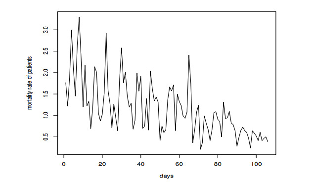
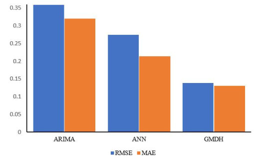
Statistical modeling and forecasting of time-to-events data are crucial in every applied sector. For the modeling and forecasting of such data sets, several statistical methods have been introduced and implemented. This paper has two aims, i.e., (i) statistical modeling and (ii) forecasting. For modeling time-to-events data, we introduce a new statistical model by combining the flexible Weibull model with the Z-family approach. The new model is called the Z flexible Weibull extension (Z-FWE) model, where the characterizations of the Z-FWE model are obtained. The maximum likelihood estimators of the Z-FWE distribution are obtained. The evaluation of the estimators of the Z-FWE model is assessed in a simulation study. The Z-FWE distribution is applied to analyze the mortality rate of COVID-19 patients. Finally, for forecasting the COVID-19 data set, we use machine learning (ML) techniques i.e., artificial neural network (ANN) and group method of data handling (GMDH) with the autoregressive integrated moving average model (ARIMA). Based on our findings, it is observed that ML techniques are more robust in terms of forecasting than the ARIMA model.
Citation: Rashad A. R. Bantan, Zubair Ahmad, Faridoon Khan, Mohammed Elgarhy, Zahra Almaspoor, G. G. Hamedani, Mahmoud El-Morshedy, Ahmed M. Gemeay. Predictive modeling of the COVID-19 data using a new version of the flexible Weibull model and machine learning techniques[J]. Mathematical Biosciences and Engineering, 2023, 20(2): 2847-2873. doi: 10.3934/mbe.2023134
Statistical modeling and forecasting of time-to-events data are crucial in every applied sector. For the modeling and forecasting of such data sets, several statistical methods have been introduced and implemented. This paper has two aims, i.e., (i) statistical modeling and (ii) forecasting. For modeling time-to-events data, we introduce a new statistical model by combining the flexible Weibull model with the Z-family approach. The new model is called the Z flexible Weibull extension (Z-FWE) model, where the characterizations of the Z-FWE model are obtained. The maximum likelihood estimators of the Z-FWE distribution are obtained. The evaluation of the estimators of the Z-FWE model is assessed in a simulation study. The Z-FWE distribution is applied to analyze the mortality rate of COVID-19 patients. Finally, for forecasting the COVID-19 data set, we use machine learning (ML) techniques i.e., artificial neural network (ANN) and group method of data handling (GMDH) with the autoregressive integrated moving average model (ARIMA). Based on our findings, it is observed that ML techniques are more robust in terms of forecasting than the ARIMA model.

| [1] | M. Gupta, A. Abdelmaksoud, M. Jafferany, T. Lotti, R. Sadoughifar, M. Goldust, COVID-19 and economy, Dermatologic Ther., 33 (2020), e13329. https://doi.org/10.1111/dth.13329 |
| [2] |
S. Rashid, S. S. Yadav, Impact of COVID-19 pandemic on higher education and research, Indian J. Hum. Dev., 14 (2020), 340–343. https://doi.org/10.1177/0973703020946700 doi: 10.1177/0973703020946700

|
| [3] |
K. S. Khan, M. A. Mamun, M. D. Griffiths, I. Ullah, The mental health impact of the COVID-19 pandemic across different cohorts, Int. J. Mental Health Addict., 20 (2022), 380–386. https://doi.org/10.1007/s11469-020-00367-0 doi: 10.1007/s11469-020-00367-0
|
| [4] |
P. Seetharaman, Business models shifts: Impact of COVID-19, Int. J. Inf. Manage., 54 (2020), 102173. https://doi.org/10.1016/j.ijinfomgt.2020.102173 doi: 10.1016/j.ijinfomgt.2020.102173
|
| [5] |
H. Wardle, C. Donnachie, N. Critchlow, A. Brown, C. Bunn, F. Dobbie, et al., The impact of the initial COVID-19 lockdown upon regular sports bettors in Britain: Findings from a cross-sectional online study, Addict. Behav., 118 (2021), 106876. https://doi.org/10.1016/j.addbeh.2021.106876 doi: 10.1016/j.addbeh.2021.106876
|
| [6] |
S. Jaipuria, R. Parida, P. Ray, The impact of COVID-19 on tourism sector in India, Tourism Recreation Res., 46 (2021), 245–260. https://doi.org/10.1080/02508281.2020.1846971 doi: 10.1080/02508281.2020.1846971
|
| [7] | M. Bebbington, C. D. Lai, R. Zitikis, A flexible Weibull extension, iReliab. Eng. Syst. Saf., 92 (2007), 719–726. https://doi.org/10.1016/j.ress.2006.03.004 |
| [8] | A. El-Gohary, A. H. El-Bassiouny, M. El-Morshedy, Exponentiated flexible Weibull extension distribution, Int. J. Math. Appl., 3 (2015), 1–12. Available from: http://ijmaa.in/index.php/ijmaa/article/view/440. |
| [9] | A. El-Gohary, A. H. El-Bassiouny, M. El-Morshedy, Inverse flexible Weibull extension distribution. Int. J. Comput. Appl., 115 (2015), 46–51. https://doi.org/10.5120/20127-2211 |
| [10] | M. A. El-Damcese, A. Mustafa, B. S. El-Desouky, M. E. Mustafa, The Kumaraswamy flexible Weibull extension, Int. J. Math. Appl., 4 (2016), 1–14. Available from: http://ijmaa.in/index.php/ijmaa/article/view/540. |
| [11] | Z. Ahmad, E. Mahmoudi, O. Kharazmi, On modeling the earthquake insurance data via a new member of the TX family, Comput. Intell. Neurosci., 2020 (2020). https://doi.org/10.1155/2020/7631495 |
| [12] |
E. Seneta, Karamata's characterization theorem, feller and regular variation in probability theory, Publ. Inst. Math., 71 (2002), 79–89. https://doi.org/10.2298/PIM0271079S doi: 10.2298/PIM0271079S
|
| [13] | W. Glänzel, A characterization theorem based on truncated moments and its application to some distribution families, in Mathematical Statistics and Probability Theory, (1987), 75–84. https://doi.org/10.1007/978-94-009-3965-3_8 |
| [14] |
W. Glänzel, Some consequences of a characterization theorem based on truncated moments, Statistics, 21 (1990), 613–618. https://doi.org/10.1080/02331889008802273 doi: 10.1080/02331889008802273
|
| [15] | G. G. Hamedani, On certain generalized gamma convolution distributions $\bf II$, Tech. Rep., (2013), 484. |
| [16] |
H. M. Almongy, E. M. Almetwally, H. M. Aljohani, A. S. Alghamdi, E. H. Hafez, A new extended Rayleigh distribution with applications of COVID-19 data, Results Phys., 23 (2021), 104012. https://doi.org/10.1016/j.rinp.2021.104012 doi: 10.1016/j.rinp.2021.104012
|
| [17] |
M. Qi, G. P. Zhang, An investigation of model selection criteria for neural network time series forecasting, Eur. J. Oper. Res., 132 (2001), 666–680. https://doi.org/10.1016/S0377-2217(00)00171-5 doi: 10.1016/S0377-2217(00)00171-5
|
| [18] |
M. Khashei, M. Bijari, An artificial neural network (p, d, q) model for timeseries forecasting, Expert Syst. Appl., 37 (2010), 479–489. https://doi.org/10.1016/j.eswa.2009.05.044 doi: 10.1016/j.eswa.2009.05.044
|
| [19] |
V. Ş. Ediger, S. Akar, ARIMA forecasting of primary energy demand by fuel in Turkey, Energy Policy, 35 (2007), 1701–1708. https://doi.org/10.1016/j.enpol.2006.05.009 doi: 10.1016/j.enpol.2006.05.009
|
| [20] | M. Khashei, M. Bijari, Which methodology is better for combining linear and non-linear models for time series forecasting? Int. J. Ind. Syst. Eng., 4 (2011), 265–285. Available from: file:///C:/Users/97380/Downloads/111420120405-1.pdf. |
| [21] | M. Qurban, X. Zhang, H. M. Nazir, I. Hussain, M. Faisal, E. E. Elashkar, et al., Development of hybrid methods for prediction of principal mineral resources, Math. Probl. Eng., 2021 (2021). https://doi.org/10.1155/2021/6362660 |
| [22] |
G. P. Zhang, Time series forecasting using a hybrid ARIMA and neural network model, Neurocomputing, 50 (2003), 159–175. https://doi.org/10.1016/S0925-2312(01)00702-0 doi: 10.1016/S0925-2312(01)00702-0
|
| [23] |
M. Khashei, Z. Hajirahimi, A comparative study of series arima/mlp hybrid models for stock price forecasting, Commun. Stat.- Simul. Comput., 48 (2019), 2625–2640. https://doi.org/10.1080/03610918.2018.1458138 doi: 10.1080/03610918.2018.1458138
|
| [24] |
P. Ravisankar, V. Ravi, Financial distress prediction in banks using Group Method of Data Handling neural network, counter propagation neural network and fuzzy ARTMAP, Knowledge Based Syst., 23 (2010), 823–831. https://doi.org/10.1016/j.knosys.2010.05.007 doi: 10.1016/j.knosys.2010.05.007
|
| [25] |
F. X. Diebold, R. S. Mariano, Comparing predictive accuracy, J. Bus. Econ. Stat., 13 (1995), 253–263. https://doi.org/10.1080/07350015.1995.10524599 doi: 10.1080/07350015.1995.10524599
|

Figures(8) / Tables(8)

Rashad A. R. Bantan, Zubair Ahmad, Faridoon Khan, Mohammed Elgarhy, Zahra Almaspoor, G. G. Hamedani, Mahmoud El-Morshedy, Ahmed M. Gemeay. Predictive modeling of the COVID-19 data using a new version of the flexible Weibull model and machine learning techniques[J]. Mathematical Biosciences and Engineering, 2023, 20(2): 2847-2873. doi: 10.3934/mbe.2023134


 DownLoad: