A region-adaptive non-local denoising algorithm for low-dose computed tomography images

1.   Introduction

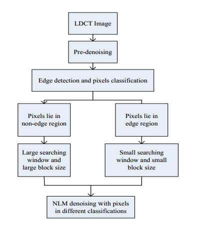
With the wide use of X-ray computed tomography (CT) in clinics, the risk of X-ray radiation-induced genetic, cancerous and other diseases is of great concern to patients and operators alike ^[1,2,3]. Low-dose computed tomography (LDCT) is an effective technique to reduce patients' radiation exposure and related hazards. However, with the reduction in dose, large increases in speckled noise and artifacts occur, resulting in seriously degraded reconstructed images. Three research methods that address this problem include projection data denoising, iterative reconstruction and post-processing methods. Among these three methods, post-processing removes noise and artifacts directly from reconstructed CT images. Moreover, it has good compatibility with existing hospital CT equipment.

Over the last few decades, a large number of image denoising algorithms have been proposed. These algorithms can be divided into two categories, traditional algorithms and deep learning algorithms. Kang et al. ^[4] introduced deep learning into low-dose CT images, initiating extensive research on deep learning in this direction. Chen et al. combined a convolutional neural network with residual encoder and decoder, and they proposed the classic RED-CNN algorithm ^[5]. Yang et al. ^[6] used Wasserstein distance in an adversarial generative network and introduced VGG-19 to calculate visual loss, which had good effect in the application of low-dose CT images. Chen et al. ^[7] combined a low-dose CT image denoising task with detection to achieve good results. Li et al. ^[8] improved the performance of the denoising network by introducing the residual attention module. Bera and Biswas ^[9] used image neighborhood information, noise characteristics, local details and other information to improve the adversarial generation network from the convolution module, loss function and discriminant function, respectively. The successful application of deep learning in low-dose CT images is remarkable. However, deep learning algorithms depend largely on the data, which is difficult for clinical LDCT images. In addition, deep learning models have poor interpretation and weak generalization ability now.

Among the traditional methods, patch-based algorithms that make use of local and non-local self-similarities in images have shown excellent performance ^{[10,11,12,13]}, the non-local means (NLM) method being a typical example of this type of algorithm. By using repetitive structures and redundant information in images, the NLM method can remove noise by averaging pixels with similar structures in a non-local neighborhood ^[14]. Owing to its excellent performance, the NLM algorithm has been widely applied to CT images. Liu et al. proposed a large-scale NLM (LNLM) method for LDCT images ^[15], further improving the LNLM method by adding the process of artifact suppression ^[16]. Li et al. proposed an adaptive NLM filter, in which the local noise level of the CT image was estimated to modify the classic NLM algorithm, achieving good performance on CT images ^[17]. Zhang et al. proposed an adaptive NLM algorithm, based on a local principle neighborhood, which exhibited good performance in noise and artifact reduction in LDCT images ^[18].

Another prior understanding of an image is that there are always several regions with different characteristics in an image—that is, smooth, edge and texture regions. However, in the classic NLM algorithm, a fixed patch size and search window of fixed size are used for all pixels in the entire image, limiting the performance of this method, especially in edge-included regions. Several improved versions of the original NLM have been proposed in recent years. By taking advantage of the local geometry of the image, Deledalle et al. proposed replacing square patches with various shapes to calculate the weights of neighboring pixels ^[19]. Khellah proposed an improved NLM method for texture image denoising by using the dominant neighborhood structure to determine the most similar pixels surrounding any given pixel within the search window ^[20]. Similarly, an NLM image-denoising method based on a local binary descriptor (LBD) was proposed in ^[21]. These algorithms selected similar pixels and excluded dissimilar ones by using different features in a fixed square search window.

Some researchers have improved the NLM algorithm by employing an adaptive search window. A modified NLM algorithm was proposed, in which the search window size was adaptively selected based on gray level differences ^[22]. This study demonstrated that a large search window could be beneficial in removing noise for pixels in a smooth region, with a small search window size being suitable for pixels in non-smooth regions. Liu et al. proposed an improved block-matching and 3D filtering (BM3D) approach that searched for candidate matching blocks along the edge directions ^[23].

By considering the advantages of the above-mentioned algorithms, an improved NLM method is proposed for LDCT image denoising in this study. In the proposed algorithm, an adaptive searching window and adaptive filtering are used in different regions for image denoising. Specifically, in smooth regions, a large isotropic square search window is selected to search for similar candidates, a large block size being used to calculate the weight coefficients. In the edge-included regions, the weight coefficients are calculated using a small block size in a small searching window. Moreover, to improve the removal of streak artifacts and speckle noise, the smoothing parameters for denoising are adaptively changed according to the noise intensity.

The remainder of this paper proceeds as follows: Section 2 briefly introduces the classic NLM algorithm and the principle of bidirectional chain codes. Section 3 presents the proposed denoising algorithm in detail. Section 4 analyzes parameter selection, presents the experimental results and compares the proposed method with several related algorithms. Finally, Section 5 concludes the paper.

2.   NLM denoising algorithm

The problem of denoising can be mathematically shown by estimating the latent clean image $\mathit{\boldsymbol{X}}$ from the noise-degraded observation model:

where $\mathit{\boldsymbol{V}}$ is the additive noise. The estimated pixel values can be calculated using the weighted average of all gray values in the entire image or a predefined non-local search window. It can be expressed as

where $\mathit{\boldsymbol{Y}}$ is the noisy image, $\mathit{\boldsymbol{\hat X}}$ is the denoised image, $num$ is the total number of pixels in $\mathit{\boldsymbol{Y}}$, $\mathit{\boldsymbol{Y}}(j)$ is the pixel intensity at position $j$, and $w(i, j)$ is the weight coefficient calculated by

where $|| \cdot ||_{2, a}^2$ is the Gaussian weighted Euclidean distance, ${N_k}$ is the patch centered at $k$, and $h$ is a smoothing parameter used to control the amount of denoising.

3.   Proposed methods

In the classic NLM algorithm, a fixed isotropic search window is used for all pixels in the entire image. This method has limitations in image denoising, especially for edge-included regions. The basic idea of our proposed algorithm is to select adaptive searching windows and adaptive filter parameters based on the region property for the calculation of weight coefficients. Specifically, in smooth regions, large isotropic searching windows and large filter parameters are selected for better denoising and smoothing. In edge-included regions, small searching windows and small filter parameters are selected for edge preservation. In the proposed method, to distinguish the edge region from that contaminated by streak artifacts, the edge-included regions are extracted based on the grayscale category information of each pixel. In the non-edge region, the filter parameter is adjusted adaptively by means of intuitionistic fuzzy divergence (IFD), which reflects the intensity of the streak artifact.

The proposed algorithm has three main steps, as shown in Figure 1, the details of which are described below.

Figure 1.  A block diagram of the proposed algorithm.

DownLoad: Full-Size Img PowerPoint

3.1.   Pixel classification and edge extraction

In this study, the edge-included and non-edge regions are distinguished based on the classification information of local blocks. For each pixel in an image, we select a 3 × 3 patch and align it to a vector. The pixels centered at each block are then divided into K categories using the K-means clustering method. The classification result using the K-means clustering method is sensitive to the selection of the initial point and the noise. To reduce the influence of noise and obtain rich edge information, the LDCT image is preprocessed using the classic NLM algorithm. In addition, we determined the initial points and the number of categories based on experience and a statistical histogram of the image. The histograms of the three images are shown in the second column in Figure 2. We can see that the histogram of the preprocessed image in Figure 2(c1) is closer to the truth than that of the LDCT image. There are five to six major gray levels in the image. According to the histogram information, we experiencedly selected six points in the preprocessed image as the initial values, as shown in Figure 3(a). Following that, pixels in the preprocessed image are classified into six groups, as shown in Figure 3(b)−(g). The classification results are shown in Figure 3(h). Finally, the gradient modulus of each pixel in the classification image is calculated. The location where the gradient modulus is not equal to zero belongs to the edge region.

Figure 2.  The edge detection results of the Shepp-Logan phantom. In the first column, from top to bottom, they are the Shepp-Logan phantom simulation, the corresponding LDCT image and the pre-processed image using the NLM method. The second column is the corresponding histograms of the images in the first column. The third colum includes the corresponding edge images of the images in first column using the Sobel operator. The fourth column includes the detected edge images using the Canny operator. The fifth column includes the detected edge images using the IFD method in this paper.

DownLoad: Full-Size Img PowerPoint

Figure 3.  Display of pixel classification display.

DownLoad: Full-Size Img PowerPoint

Figure 2 shows the results of edge detection on the Shepp-Logan phantom image using different methods. From top to bottom, the images in the first column are the Shepp-Logan phantom simulation, the corresponding LDCT image reconstructed from simulated noisy sinograms by using the filtered back-projection (FBP) method and the preprocessed image denoised using the NLM method. The images in the third to the fifth columns are the detected edge images of those in the first column using the Sobel operator, the Canny operator and the IFD method (it will be described in Section 3.2.1), respectively. It can be seen that the edges in the images in the fourth column are richer and more accurate than those in the second and third columns, the edge extraction method used in this study being more resilient to streak artifacts—that is, the detected edge information in Figure 2(c4) is closer to that in Figure 2(a4).

Based on the edge extraction results, for non-edge regions, a large search window and block size were used, whereas for edge included regions, the search window and block size were both small.

3.2.   Adaptive filter parameter

In the NLM algorithm, the selection of filtering parameters has a significant influence on the denoising results. However, in an LDCT image, a large filter parameter can reduce streak artifacts, but accompanying image blurring occurs. Meanwhile, a small filter parameter is not conducive to noise removal, especially for streak artifacts. For better denoising performance, in this study, the filter parameter for each pixel is adjusted adaptively by means of IFD between a smooth template and a local block centered at the current pixel.

3.2.1.   Intuitionistic fuzzy divergence

Intuitionistic fuzzy divergence (IFD) is a method for measuring the degree of similarity between two fuzzy sets. The larger the IFD distance is, the more dissimilar the two sets are. The definition of IFD is

where $A$ and $B$ are two fuzzy sets, ${\mu _A}({a_{ij}})$ represents the degree of membership of element ${a_{ij}}$ in set $A$, ${\mu _B}({b_{ij}})$ represents the degree of membership of element ${b_{ij}}$ in set $B$, ${\pi _A}({a_{ij}})$ is the hesitation degree of element ${a_{ij}}$ to set $A$, and ${\pi _B}({b_{ij}})$ is the hesitation degree of element ${b_{ij}}$ to set $B$.

3.2.2.   Adaptive filter parameter based on IFD

We define a template of size 3 × 3, in which all elements are zero. The template represents the smooth region, which we denote as $O$. For each pixel ${x_0}$ in the LDCT image, the local block of size 3 × 3 is denoted as $P$. $O$ and $P$ are the two fuzzy sets used for the LDCT image-denoising problem.

In this paper, we calculate the IFD at $({i_{0, }}{j_0})$ by using the following equation:

where $({i_{0, }}{j_0})$ is the coordinate of the center pixel ${x_0}$ in $P$, ${a_{ij}}$ is the element in $P$, and ${o_{ij}}$ is the corresponding pixel in the template $O$.

In Eq (4), the membership function and the hesitation degree function are key factors in calculating the IFD between the two sets. In this paper, a membership function that uses both gradient information and local variance information is proposed for pixels in set $P$.

where ${\sigma ^2}$ is the normalized local variance of pixel ${a_{ij}}$.

The hesitation degree function is

where ${p_1}$ is a coefficient. In this paper, ${p_1} = 0.5$.

For pixels in set $O$, the membership function $\mu ({o_{ij}}) = 0$, and the hesitation degree function is

where ${p_2}$ is a coefficient. In this paper, ${p_2} = 0.5$.

Based on Eqs (4)−(9), the IFD for all pixels in the LDCT image can be calculated. For each pixel, the greater the IFD value is, the higher the pixel is polluted by streak artifacts and speckle noise. Accordingly, an adaptive filter parameter is proposed as follows:

where $h(i, j)$ is the filter parameter for the pixel located at $(i, j)$, $\delta$ is the standard deviation of noise, and $IFD({I}_{ij}, O)$ is the IFD between the template $O$ and the local block centered at $(i, j)$ in the image ${I_{ij}}$.

3.3.   Adaptive filter parameter

Based on Eq (3), the weight coefficient can be calculated in its search window. However, a large number of pixels that are significantly different from the center pixel values may be included in the search window, especially in the regions near the edge. To improve the denoising performance, dissimilar pixels are removed based on the pixel classification information obtained in step 1 and described in Section 3.1. In Figure 4(a), the center pixel circled in blue is the current pixel to be denoised. It can be seen that there are many points that have significantly different gray values from the center point in the searching window. Figure 4(b) shows the pixel classification results. By removing pixels in different classifications, the remaining black pixels in Figure 4(c) are similar pixels used for the denoising of the center pixel.

Figure 4.  (a) A pixel and its searching window, (b) the classification information of pixels in the searching window, (c) similar pixels used for denoising of the center pixel.

DownLoad: Full-Size Img PowerPoint

4.   Experimental results

In this section, we evaluated the performance of the proposed method through experiments on the Shepp-Logan head phantom, as shown in Figure 4(a). The denoising results obtained using our proposed method were compared to several related methods, including the NLM method, the TV algorithm ^[24] and the improved NLM algorithm in ^[22] (denoted as GLD-NLM).

Two evaluation criteria were used in this study to objectively evaluate the quality of the denoised images. The first is the peak-signal-to-noise ratio (PSNR), which is the most common and widely used objective evaluation standard for image quality. The PSNR between two images $X$ and $Y$, both of size $M \times N$, can be calculated as follows:

The other criterion is that of structural similarity (SSIM). The SSIM between windows $x$ and $y$ of size $W \times W$ can be defined as

where ${\mu _x}$ is the average of $x$, ${\mu _y}$ is the average of $y$, $\sigma _x^2$ is the variance of $x$, $\sigma _y^2$ is the variance of $y$, ${\sigma _{xy}}$ is the covariance of $x$ and $y$, and the positive constants ${c_1}$ and ${c_2}$ are used to avoid a null denominator.

4.1.   Phantom study

4.1.1.   Visual assessment

In the classic NLM algorithm, the block size was 7 × 7, the searching window was 21 × 21, and the filter parameter was $h = \sigma$. In the GLD-NLM algorithm, the parameters were selected based on ^[22]. In the proposed method, the large block size was 9 × 9, the small block size was 5 × 5, the large searching window was 29 × 29, and the small searching window was 15 × 15. The filter parameter $h$ was calculated using Eq (10). The grouping number K in the edge extraction stage was set empirically according to the LDCT images. In our experiment it was 6 for both the Shepp-Logan head phantom and the clinal image. The noise variance was selected according to experiments.

In this paper, a non-stationary Gaussian distribution model is used to simulate noise in projection domain.

where ${m_i}$ is the mean value calculated by (15), ${\sigma _i}$ is variance calculated by (16), ${a_{ij}}$ is the element of the system matrix, and ${f_i}$ and $\eta$ are parameters that depend on the configuration of the CT device system.

The simulated low dose Shepp-Logan phantoms under different dose levels are shown in Figure 5. Figure 5(a) is the simulated clean image, and Figure 5(b)−(f) shows the reconstructed LDCT image from the simulated noisy sinogram using the FBP method (Hanning filter with cutoff at 80% Nyquist frequency). The parameters for the LDCT images are (b) ${f_i} = 50$, $\eta = 22000$, (c) ${f_i} = 100$, $\eta = 22000$, (d)${f_i} = 200$, $\eta = 22000$, (e)${f_i} = 800$, $\eta = 62000$, (f)${f_i} = 300$, $\eta = 22000$, respectively.

Figure 5.  Simulated Shepp-Logan phantom in different low dose levels.

DownLoad: Full-Size Img PowerPoint

The denoising results by using NLM, TV, GLD-NLM and the proposed method are shown in Figure 6. As can be seen in the two charts, the proposed method shows more proficiency in image denoising.

Figure 6.  Comparison of denoising performances on the images in Figure 4 among NLM, TV, GLD-NLM and the proposed method. (a) PSNR, (b) SSIM.

DownLoad: Full-Size Img PowerPoint

Figures 7–9 show the denoised results of the low dose image in Figure 5(d) in order to further compare the visual effects of the denoised images. Figure 7(c)–(f) shows the denoising results obtained using the NLM, TV, GLD-NLM and proposed methods, respectively. Figures 8 and 9 show the partially enlarged details of the two regions of interest—that is, ROI1 and ROI2—marked by red rectangles in Figure 7(a). The TV model, as a classical image restoration method, has been successfully applied in LDCT images and achieved competitive denoising results; however, it could not achieve good results in noise removal and detail protection simultaneously. In Figure 8(d), the details are significantly blurred. In Figure 9(d), there is an obvious block effect near the edge region. The classic NLM algorithm is superior in protecting image details; however, the streak artifacts are protected at the same time. As shown in Figure 7(c), many streak artifacts remain in the denoised image. From the partially enlarged images in Figures 8(c) and 9(c), it can be seen that regions that were originally seriously contaminated by streak artifacts in the LDCT image are still full of noise in the denoised image. The GLD-NLM algorithm performs well for Gaussian noise denoising; however, for streak artifacts and speckle noise in LDCT images, its performance is poor. By contrast, the proposed method performs well in LDCT image denoising. From Figures 8(f) and 9(f), it can be seen that the noise is almost removed, the image edges being relatively clear.

Figure 7.  Comparison of several related algorithms. (a) The original Shepp-Logan phantom, (b) the reconstructed LDCT image from simulated noisy sinogram using the FBP method (Hanning filter with cutoff at 80% Nyquist frequency), (c) NLM, (d) TV, (e) GLD-NLM, (f) proposed method.

DownLoad: Full-Size Img PowerPoint

Figure 8.  Comparison of partially enlarged detail ROI1. (a) Original Shepp-Logan phantom, (b) LDCT image, (c) NLM, (d) TV, (e) GLD-NLM, (f) proposed method.

DownLoad: Full-Size Img PowerPoint

Figure 9.  Comparison of partially enlarged detail ROI2. (a) Original Shepp-Logan phantom, (b) LDCT image, (c) NLM, (d) TV, (e) GLD-NLM, (f) proposed method.

DownLoad: Full-Size Img PowerPoint

4.1.2.   Quantitative assessment

The objective evaluations of the NLM, TV, GLD-NLM and proposed methods are shown in Table 1. The PSNR and SSIM values produced using these methods for the Shepp-Logan phantom in Figure 4(c) were calculated using Eqs (11)–(13), the maximum values among all the methods being highlighted in bold. As can be seen from the table, both the PSNR and SSIM values of the proposed method are the maximum values.

Table 1.  Comparison of the denoising outcomes of the Shepp-Logan phantom.

Shepp-Logan phantom	Whole		ROI1		ROI2
	PSNR	SSIM	PSNR	SSIM	PSNR	SSIM
Noisy	18.3171	0.2148	16.3667	0.6807	14.323	0.4538
NLM	23.8261	0.4975	21.9658	0.8193	19.9681	0.6648
TV	22.4618	0.5633	21.2553	0.7827	20.9558	0.8061
NLM-GLD	22.7169	0.5015	21.4792	0.7732	18.6847	0.617
Proposed method	24.1361	0.5822	22.4887	0.8427	23.0489	0.9069

---

 | Show Table

DownLoad: CSV

4.2.   Clinical data

In this section, a low-dose clinical abdominal image slice (as shown in Figure 9(a1)) obtained from the Mayo Clinic (USA) ^[25] was used to verify the effectiveness and feasibility of the proposed denoising algorithm. The slice was obtained from a patient with liver cancer, and the image size was 512 × 512.

4.2.1.   Visual assessment

The denoising results obtained using the proposed method were compared with those obtained using the NLM, GLD-NLM and TV methods. The experimental results are shown in Figure 10(a1)−(f1). The enlarged images of the region of interest (ROI)—in this case referring to the liver tumor marked with a white box—are shown in Figure 10(a2)−(f2). Figure 10(a1) shows a low-dose clinical abdominal image slice, with Figure 10(b1) showing a high-dose clinical abdominal image slice. Figure 10(c1)−(f1) shows the denoising results using NLM, GLD-NLM, TV and proposed methods, respectively. We can see that the images obtained using the NLM and GLD-NLM methods still suffer from noise and artifacts. The TV method achieved good results in noise removal and detail protection, but there is an obvious blocking effect in noisy areas. By contrast, the denoised image using the proposed method is significantly reduced, and the image edge is relatively clear.

Figure 10.  Comparison of denoised results of various algorithms: (a) LDCT, (b) standard dose CT, (c) NLM, (d) GLD-NLM, (e) TV and (f) proposed method.

DownLoad: Full-Size Img PowerPoint

4.2.2.   Quantitative assessment

To evaluate the quality of the denoised image, PSNR and SSIM techniques were used to quantitatively evaluate the whole clinical abdominal image and the area of interest (liver tumor). The definitions of PSNR and SSIM are given in Eqs (11)−(13). In addition, six other ROIs (designated by the red square) in Figure 7(a1) were selected for quantitative description analysis. Three flat areas are marked ROI1, ROI2 and ROI3, and three edge areas are labeled ROI4, ROI5 and ROI6.

Table 2 lists the PSNR and SSIM values of the original LDCT images, the ROIs after applying the NLM, GLD-NLM, TV and proposed methods. It can be seen that the proposed algorithm has the largest PSNR value and the second largest SSIM value for the whole image, the largest PSNR value in all ROIs and the largest SSIM value in most ROIs. Clearly, the proposed method has a good trade-off between noise reduction and edge preservation.

Table 2.  PSNR and SSIM evaluation of the original LDCT images, standard dose CT images and the processed LDCT images.

	LDCT		NLM		NLM-GLD		TV		Proposed
	PSNR	SSIM	PSNR	SSIM	PSNR	SSIM	PSNR	SSIM	PSNR	SSIM
Whole	34.86	0.82	37.76	0.91	37.45	0.90	36.59	0.93	38.23	0.92
Cancer	26.52	0.70	29.76	0.83	29.06	0.81	29.00	0.89	31.78	0.90
ROI1	26.76	0.71	29.59	0.83	28.95	0.80	29.12	0.88	31.76	0.92
ROI2	26.19	0.65	30.41	0.84	29.36	0.79	29.34	0.90	31.64	0.90
ROI3	26.20	0.70	27.98	0.77	27.77	0.77	29.12	0.86	30.78	0.89
ROI4	28.05	0.85	32.43	0.94	31.89	0.93	29.71	0.94	33.27	0.95
ROI5	26.05	0.74	29.19	0.85	28.72	0.83	29.36	0.92	29.82	0.86
ROI6	27.90	0.82	30.96	0.92	30.81	0.91	30.51	0.93	31.01	0.93

---

 | Show Table

DownLoad: CSV

4.3.   Calculation time

The experiments in this paper were implemented in MATLAB 2010b 32bit on a personal computer equipped with a CPU G620 @2.60 GHz and 8 GB memory. The running times of different methods are listed in Table 3. The data are the average times for 256 × 256 simulated LDCT images. The running time of the TV algorithm is related to the iteration error or the number of iterations. From Table 3, when the iteration error is set as 1e-5, the running time is 15.04 s. When the iteration error is set as 1e-4, the running time reduced by 75%. In this paper, the former is used because of the higher image quality. The NLM-based methods are time-consuming. This is mainly because of the heavy calculation of the weight matrix in formula (3). In the NLM-GLD method and our proposed method, basic NLM algorithm is used for preprocessing. There is no doubt that using it directly will greatly increase the running time. By removing the Gaussian weighed kernel, the running time of NLM-GLD is reduced sharply, although the NLM algorithm is used almost twice. In the proposed method, the calculation of distance between two similar patches is changed into the formula (17), as follows. By calculating the first two terms ahead of the for loop structure, the running time of the proposed method reduced to 22.03 s.

Table 3.  Running time (in seconds) of different methods.

Method	NLM	TV	NLM-GLD	Proposed method
Time (s)	92.87	15.04	56.26	22.03

---

 | Show Table

DownLoad: CSV

where $|| \cdot ||_{2, a}^2$ is the Gaussian weighted Euclidean distance, ${N_k}$ is the patch centered at pixel $k$, and $\mathit{\boldsymbol{Y}}\left( {\mathop N\nolimits_i } \right) \otimes \mathit{\boldsymbol{Y}}\left( {\mathop N\nolimits_j } \right)$ denotes the convolution operation of $\mathit{\boldsymbol{Y}}\left( {\mathop N\nolimits_i } \right)$ and $\mathit{\boldsymbol{Y}}\left( {\mathop N\nolimits_j } \right)$.

5.   Discussion

Although similar ideas are adopted in our paper and in ^[22], that is, a large search window could be beneficial in removing noise for pixels in a smooth region, a small search window size being suitable for pixels in non-smooth regions, there are several differences between the two methods. In ^[22], the search window size was adaptively selected based on gray level differences. In our method, the pixels are classified into several regions according to the K-means algorithm. In reference ^[22], the searching window is square for each pixel, and all pixels in the searching window are involved in the calculation of weight coefficients. However, in our method, in the non-smooth regions, the non-local similar pixels in the searching window are filtered again based on edge information. Only pixels along with the edge are used to calculate the weight coefficients. It is beneficial for protecting the edge details in the image. Moreover, the smoothing parameters for denoising are adaptively changed according to the noise intensity in the LDCT images. From the experimental results, we can see that our method outperforms the method in ^[22].

6.   Conclusions

In this paper, we proposed a region-adaptive NLM denoising method for LDCT images. In the proposed method, the size of the searching window and block size were adaptively selected for different regions based on pixel classification results. For non-edge regions, a large search window and block size were used for better denoising. For edge-included regions, a small search window and block size were used for edge protection. Further, we filtered the pixels in the search window based on pixel classification results, removing pixels of different categories and retaining pixels of the same category. Moreover, the filter parameter was adjusted adaptively based on the severity of the noise, by means of IFD. Overall, through all of the above efforts, denoising performance was improved. Experiments on the Shepp-Logan phantom showed that the proposed method was effective, outperforming several related denoising methods. The main limitation is that the parameters in our method are not all decided automatically. For example, the grouping number K in the edge extraction stage is set empirically according to the LDCT images. Although the running time has been reduced greatly in our method, there is still a gap for real-time applications. In the future works, automatic adaptive parameters and multiscale characteristic will be studied to combine with our method to further improve denoising performance. The running time can be further improved by optimizing the code structure.

Acknowledgments

This work was supported in part by the National Natural Science Foundation under Grant 11605160, in part by the Natural Science Foundation of Shanxi Province under Grant 201901D211246 and 201901D111031, in part by the Research Project Supported by the Shanxi Scholarship Council of China under Grant 2021-111 and in part by the Shanxi Province Universities Science and Technology Innovation Project under Grant 2020L0051.

Conflict of interest

The authors declare there is no conflict of interest.