Magneto-Acousto-Electrical Tomography (MAET) is a multi-physics coupling imaging modality that integrates the high resolution of ultrasound imaging with the high contrast of electrical impedance imaging. However, the quality of images obtained through this imaging technique can be easily compromised by environmental or experimental noise, thereby affecting the overall quality of the imaging results. Existing methods for magneto-acousto-electrical image denoising lack the capability to model local and global features of magneto-acousto-electrical images and are unable to extract the most relevant multi-scale contextual information to model the joint distribution of clean images and noise images. To address this issue, we propose a Dual Generative Adversarial Network based on Attention Residual U-Net (ARU-DGAN) for magneto-acousto-electrical image denoising. Specifically, our model approximates the joint distribution of magneto-acousto-electrical clean and noisy images from two perspectives: noise removal and noise generation. First, it transforms noisy images into clean ones through a denoiser; second, it converts clean images into noisy ones via a generator. Simultaneously, we design an Attention Residual U-Net (ARU) to serve as the backbone of the denoiser and generator in the Dual Generative Adversarial Network (DGAN). The ARU network adopts a residual mechanism and introduces a linear Self-Attention based on Cross-Normalization (CNorm-SA), which is proposed in this paper. This design allows the model to effectively extract the most relevant multi-scale contextual information while maintaining high resolution, thereby better modeling the local and global features of magneto-acousto-electrical images. Finally, extensive experiments on a real-world magneto-acousto-electrical image dataset constructed in this paper demonstrate significant improvements in preserving image details achieved by ARU-DGAN. Furthermore, compared to the state-of-the-art competitive methods, it exhibits a 0.3 dB increase in PSNR and an improvement of 0.47% in SSIM.
Citation: Shuaiyu Bu, Yuanyuan Li, Wenting Ren, Guoqiang Liu. ARU-DGAN: A dual generative adversarial network based on attention residual U-Net for magneto-acousto-electrical image denoising[J]. Mathematical Biosciences and Engineering, 2023, 20(11): 19661-19685. doi: 10.3934/mbe.2023871
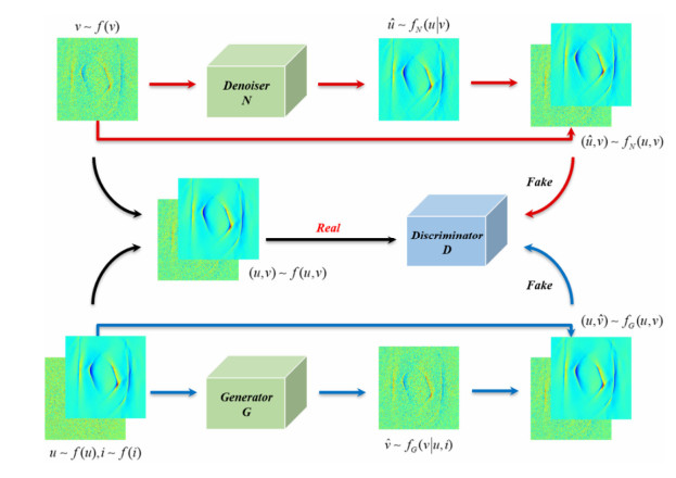
Magneto-Acousto-Electrical Tomography (MAET) is a multi-physics coupling imaging modality that integrates the high resolution of ultrasound imaging with the high contrast of electrical impedance imaging. However, the quality of images obtained through this imaging technique can be easily compromised by environmental or experimental noise, thereby affecting the overall quality of the imaging results. Existing methods for magneto-acousto-electrical image denoising lack the capability to model local and global features of magneto-acousto-electrical images and are unable to extract the most relevant multi-scale contextual information to model the joint distribution of clean images and noise images. To address this issue, we propose a Dual Generative Adversarial Network based on Attention Residual U-Net (ARU-DGAN) for magneto-acousto-electrical image denoising. Specifically, our model approximates the joint distribution of magneto-acousto-electrical clean and noisy images from two perspectives: noise removal and noise generation. First, it transforms noisy images into clean ones through a denoiser; second, it converts clean images into noisy ones via a generator. Simultaneously, we design an Attention Residual U-Net (ARU) to serve as the backbone of the denoiser and generator in the Dual Generative Adversarial Network (DGAN). The ARU network adopts a residual mechanism and introduces a linear Self-Attention based on Cross-Normalization (CNorm-SA), which is proposed in this paper. This design allows the model to effectively extract the most relevant multi-scale contextual information while maintaining high resolution, thereby better modeling the local and global features of magneto-acousto-electrical images. Finally, extensive experiments on a real-world magneto-acousto-electrical image dataset constructed in this paper demonstrate significant improvements in preserving image details achieved by ARU-DGAN. Furthermore, compared to the state-of-the-art competitive methods, it exhibits a 0.3 dB increase in PSNR and an improvement of 0.47% in SSIM.

| [1] |
P. Grasland-Mongrain, C. Lafon, Review on biomedical techniques for imaging electrical impedance, IRBM, 39 (2018), 243–250. https://doi.org/10.1016/j.irbm.2018.06.001 doi: 10.1016/j.irbm.2018.06.001

|
| [2] |
H. Wen, R. S. Balaban, The potential for hall effect breast imaging, Breast Dis., 10 (1998), 191–195. https://doi.org/10.3233/BD-1998-103-418 doi: 10.3233/BD-1998-103-418
|
| [3] |
Y. Zhou, Z. Yu, Q. Ma, G. Guo, J. Tu, D. Zhang, Noninvasive treatment-efficacy evaluation for HIFU therapy based on magneto-acousto-electrical tomography, IEEE Trans. Biomed. Eng., 66 (2018), 666–674. https://doi.org/10.1109/TBME.2018.2853594 doi: 10.1109/TBME.2018.2853594
|
| [4] |
Y. Li, G. Liu, H. Xia, Z. Xia, Numerical simulations and experimental study of magneto-acousto-electrical tomography with plane transducer, IEEE Trans. Magn., 54 (2017), 1–4. https://doi.org/10.1109/TMAG.2017.2771564 doi: 10.1109/TMAG.2017.2771564
|
| [5] |
G. Guo, J. Wang, Q. Ma, J. Tu, D. Zhang, Non-invasive treatment efficacy evaluation for high-intensity focused ultrasound therapy using magnetically induced magnetoacoustic measurement, J. Appl. Phys., 123 (2018), 154901. https://doi.org/10.1063/1.5024735 doi: 10.1063/1.5024735
|
| [6] |
M. S. Gözü, R. Zengin, N. G. Gençer, Numerical implementation of magneto-acousto-electrical tomography (MAET) using a linear phased array transducer, Phys. Med. Biol., 63 (2018), 35012. https://doi.org/10.1088/1361-6560/aa9f3b doi: 10.1088/1361-6560/aa9f3b
|
| [7] | P. Grasland-Mongrain, F. Destrempes, J. Mari, R. Souchon, S. Catheline, J. Chapelon, Acousto-electrical speckle pattern in electrical impedance tomography, in 2014 IEEE International Ultrasonics Symposium, (2014), 221–223. https://doi.org/10.1109/ULTSYM.2014.0056 |
| [8] |
L. Guo, G. Liu, H. Xia, Magneto-acousto-electrical tomography with magnetic induction for conductivity reconstruction, IEEE Trans. Biomed. Eng., 62 (2014), 2114–2124. https://doi.org/10.1109/TBME.2014.2382562 doi: 10.1109/TBME.2014.2382562
|
| [9] |
L. Kunyansky, C. P. Ingram, R. S. Witte, Rotational magneto-acousto-electric tomography (MAET): theory and experimental validation, Phys. Med. Biol., 62 (2017), 3025. https://doi.org/10.1088/1361-6560/aa6222 doi: 10.1088/1361-6560/aa6222
|
| [10] |
L. Kunyansky, A mathematical model and inversion procedure for magneto-acousto-electric tomography, Inverse Probl., 28 (2012), 035002. https://doi.org/10.1088/0266-5611/28/3/035002 doi: 10.1088/0266-5611/28/3/035002
|
| [11] |
H. Ammari, P. Grasland-Mongrain, P. Millien, L. Seppecher, J. Seo, A mathematical and numerical framework for ultrasonically-induced Lorentz force electrical impedance tomography, J. Math. Pures Appl., 103 (2015), 1390–1409. https://doi.org/10.1016/j.matpur.2014.11.003 doi: 10.1016/j.matpur.2014.11.003
|
| [12] |
Y. Li, J. Song, H. Xia, G. Liu, The experimental study of mouse liver in magneto-acousto-electrical tomography by scan mode, Phys. Med. Biol., 65 (2020), 215024. https://doi.org/10.1088/1361-6560/abb4bb doi: 10.1088/1361-6560/abb4bb
|
| [13] |
Z. Sun, G. Liu, H. Xia, S. Catheline, Lorentz force electrical-impedance tomography using linearly frequency-modulated ultrasound pulse, IEEE Trans. Ultrason. Ferroelectr. Freq. Control, 65 (2018), 168–177. https://doi.org/10.1109/TUFFC.2017.2781189 doi: 10.1109/TUFFC.2017.2781189
|
| [14] |
M. Dai, X. Chen, T. Sun, L. Yu, M. Chen, H. Lin, A 2D magneto-acousto-electrical tomography method to detect conductivity variation using multifocus image method, Sensors, 18 (2018), 2373. https://doi.org/10.3390/s18072373 doi: 10.3390/s18072373
|
| [15] |
E. Renzhiglova, V. Ivantsiv, Y. Xu, Difference frequency magneto-acousto-electrical tomography (DF-MAET): application of ultrasound-induced radiation force to imaging electrical current density, IEEE Trans. Ultrason. Ferroelectr. Freq. Control, 57 (2010), 2391–2402. https://doi.org/10.1109/TUFFC.2010.1707 doi: 10.1109/TUFFC.2010.1707
|
| [16] |
A. Montalibet, J. Jossinet, A. Matias, Scanning electric conductivity gradients with ultrasonically-induced lorentz force, Ultrason. Imaging, 23 (2001), 117–132. https://doi.org/10.1177/016173460102300204 doi: 10.1177/016173460102300204
|
| [17] |
Y. Jin, H. Zhao, G. Liu, H. Xia, Y. Li, The application of wavelet filtering method in magneto-acousto-electrical tomography, Phys. Med. Biol., 68 (2023), 145014. https://doi.org/10.1088/1361-6560/ace09c doi: 10.1088/1361-6560/ace09c
|
| [18] | S. Anwar, N. Barnes, Real image denoising with feature attention, in 2019 IEEE/CVF International Conference on Computer Vision (ICCV), (2019), 3155–3164. https://doi.org/10.1109/ICCV.2019.00325 |
| [19] | Z. Yue, H. Yong, Q. Zhao, D. Meng, L. Zhang, Variational denoising network: toward blind noise modeling and removal, in Advances in Neural Information Processing Systems, 32 (2019). Available from: https://proceedings.neurips.cc/paper_files/paper/2019/file/6395ebd0f4b478145ecfbaf939454fa4-Paper.pdf. |
| [20] |
K. Zhang, W. Zuo, Y. Chen, D. Meng, L. Zhang, Beyond a gaussian denoiser: residual learning of deep CNN for image denoising, IEEE Trans. Image Process., 26 (2017), 3142–3155. https://doi.org/10.1109/TIP.2017.2662206 doi: 10.1109/TIP.2017.2662206
|
| [21] | I. Goodfellow, J. Pouget-Abadie, M. Mirza, B. Xu, D. Warde-Farley, S. Ozair, et al., Generative adversarial nets, in Advances in Neural Information Processing Systems, 27 (2014). Available from: https://proceedings.neurips.cc/paper_files/paper/2014/file/5ca3e9b122f61f8f06494c97b1afccf3-Paper.pdf. |
| [22] | J. Chen, J. Chen, H. Chao, M. Yang, Image blind denoising with generative adversarial network based noise modeling, in 2018 IEEE/CVF Conference on Computer Vision and Pattern Recognition, (2018), 3155–3164. https://doi.org/10.1109/CVPR.2018.00333 |
| [23] | D. W. Kim, J. R. Chung, S. W. Jung, Grdn: Grouped residual dense network for real image denoising and gan-based real-world noise modeling, in 2019 IEEE/CVF Conference on Computer Vision and Pattern Recognition Workshops (CVPRW), (2019), 2086–2094. https://doi.org/10.1109/CVPRW.2019.00261 |
| [24] |
P. Grasland-Mongrain, J. M. Mari, J. Y. Chapelon, C. Lafon, Lorentz force electrical impedance tomography, IRBM, 34 (2013), 357–360. https://doi.org/10.1016/j.irbm.2013.08.002 doi: 10.1016/j.irbm.2013.08.002
|
| [25] |
Y. Li, S. Bu, X. Han, H. Xia, W. Ren, G. Liu, Magneto-acousto-electrical tomography with nonuniform static magnetic field, IEEE Trans. Instrum. Meas., 72 (2023), 1–12. https://doi.org/10.1109/TIM.2023.3244814 doi: 10.1109/TIM.2023.3244814
|
| [26] |
H. Lin, Y. Chen, S. Xie, M. Yu, D. Deng, T. Sun, et al., A dual-modal imaging method combining ultrasound and electromagnetism for simultaneous measurement of tissue elasticity and electrical conductivity, IEEE Trans. Biomed. Eng., 69 (2022), 2499–2511. https://doi.org/10.1109/TBME.2022.3148120 doi: 10.1109/TBME.2022.3148120
|
| [27] |
M. Aharon, M. Elad, A. Bruckstein, K-SVD: An algorithm for designing overcomplete dictionaries for sparse representation, IEEE Trans. Signal Process., 54 (2006), 4311–4322. https://doi.org/10.1109/TSP.2006.881199 doi: 10.1109/TSP.2006.881199
|
| [28] |
M. Elad, M. Aharon, Image denoising via sparse and redundant representations over learned dictionaries, IEEE Trans. Image Process., 15 (2006), 3736–3745. https://doi.org/10.1109/TIP.2006.881969 doi: 10.1109/TIP.2006.881969
|
| [29] | S. Gu, L. Zhang, W. Zuo, X. Feng, Weighted nuclear norm minimization with application to image denoising, in 2014 IEEE Conference on Computer Vision and Pattern Recognition, (2014), 2862–2869. https://doi.org/10.1109/CVPR.2014.366 |
| [30] | A. Buades, B. Coll, J. M. Morel, A non-local algorithm for image denoising, in 2005 IEEE Computer Society Conference on Computer Vision and Pattern Recognition (CVPR'05), 2 (2005), 60–65. https://doi.org/10.1109/CVPR.2005.38 |
| [31] |
K. Dabov, A. Foi, V. Katkovnik, K. Egiazarian, Image denoising by sparse 3-D transform-domain collaborative filtering, IEEE Trans. Image Process., 16 (2007), 2080–2095. https://doi.org/10.1109/TIP.2007.901238 doi: 10.1109/TIP.2007.901238
|
| [32] |
J. Portilla, V. Strela, M. J. Wainwright, E. P. Simoncelli, Image denoising using scale mixtures of Gaussians in the wavelet domain, IEEE Trans. Image Process., 12 (2003), 1338–1351. https://doi.org/10.1109/TIP.2003.818640 doi: 10.1109/TIP.2003.818640
|
| [33] |
L. I. Rudin, S. Osher, E. Fatemi, Nonlinear total variation based noise removal algorithms, Physica D, 60 (1992), 259–268. https://doi.org/10.1016/0167-2789(92)90242-F doi: 10.1016/0167-2789(92)90242-F
|
| [34] |
A. Barbu, Training an active random field for real-time image denoising, IEEE Trans. Image Process., 18 (2009), 2451–2462. https://doi.org/10.1109/TIP.2009.2028254 doi: 10.1109/TIP.2009.2028254
|
| [35] | K. G. G. Samuel, M. F. Tappen, Learning optimized MAP estimates in continuously-valued MRF models, in 2009 IEEE Conference on Computer Vision and Pattern Recognition, (2009), 477–484. https://doi.org/10.1109/CVPR.2009.5206774 |
| [36] |
J. Sun, M. F. Tappen, Learning non-local range Markov Random field for image restoration, CVPR 2011, (2011), 2745–2752. https://doi.org/10.1109/CVPR.2011.5995520 doi: 10.1109/CVPR.2011.5995520
|
| [37] | U. Schmidt, Half-quadratic Inference and Learning for Natural Images, Ph.D thesis, Technische University, 2017. Available from: https://tuprints.ulb.tu-darmstadt.de/id/eprint/6044. |
| [38] | U. Schmidt, S. Roth, Shrinkage fields for effective image restoration, in 2014 IEEE Conference on Computer Vision and Pattern Recognition, (2014), 2774–2781. https://doi.org/10.1109/CVPR.2014.349 |
| [39] |
Y. Chen, T. Pock, Trainable nonlinear reaction diffusion: a flexible framework for fast and effective image restoration, IEEE Trans. Pattern Anal. Mach. Intell., 39 (2017), 1256–1272. https://doi.org/10.1109/TPAMI.2016.2596743 doi: 10.1109/TPAMI.2016.2596743
|
| [40] | V. Jain, S. Seung, Natural image denoising with convolutional networks, in Advances in Neural Information Processing Systems, 21 (2008). Available from: https://proceedings.neurips.cc/paper_files/paper/2008/file/c16a5320fa475530d9583c34fd356ef5-Paper.pdf. |
| [41] | H. C. Burger, C. J. Schuler, S. Harmeling, Image denoising: can plain neural networks compete with BM3D? in 2012 IEEE Conference on Computer Vision and Pattern Recognition, (2012), 2392–2399. https://doi.org/10.1109/CVPR.2012.6247952 |
| [42] | X. Mao, C. Shen, Y. B. Yang, Image restoration using very deep convolutional encoder-decoder networks with symmetric skip connections, in Advances in Neural Information Processing Systems, 29 (2016). Available from: https://proceedings.neurips.cc/paper_files/paper/2016/file/0ed9422357395a0d4879191c66f4faa2-Paper.pdf. |
| [43] | D. Liu, B. Wen, Y. Fan, C. C. Loy, T. S. Huang, Non-local recurrent network for image restoration, in Advances in Neural Information Processing Systems, 31 (2018). Available from: https://proceedings.neurips.cc/paper_files/paper/2018/file/fc49306d97602c8ed1be1dfbf0835ead-Paper.pdf. |
| [44] | T. Plötz, S. Roth, Neural nearest neighbors networks, in Advances in Neural Information Processing Systems, 31 (2018). Available from: https://proceedings.neurips.cc/paper_files/paper/2018/file/f0e52b27a7a5d6a1a87373dffa53dbe5-Paper.pdf. |
| [45] | Z. Yue, Q. Zhao, L. Zhang, D. Meng, Dual adversarial network: toward real-world noise removal and noise generation, in Computer Vision – ECCV 2020, (2020), 41–58. https://doi.org/10.1007/978-3-030-58607-2_3 |
| [46] |
N. Mu, Z. Lyu, M. Rezaeitaleshmahalleh, J. Tang, J. Jiang, An attention residual u-net with differential preprocessing and geometric postprocessing: learning how to segment vasculature including intracranial aneurysms, Med. Image Anal., 84 (2023), 102697. https://doi.org/10.1016/j.media.2022.102697 doi: 10.1016/j.media.2022.102697
|
| [47] |
X. Liu, D. Zhang, J. Yao, J. Tang, Transformer and convolutional based dual branch network for retinal vessel segmentation in OCTA images, Biomed. Signal Process. Control, 83 (2023), 104604. https://doi.org/10.1016/j.bspc.2023.104604 doi: 10.1016/j.bspc.2023.104604
|
| [48] |
M. Versaci, G. Angiulli, P. Crucitti, D. de Carlo, F. Laganà, D. Pellicanò, et al., A fuzzy similarity-based approach to classify numerically simulated and experimentally detected carbon fiber-reinforced polymer plate defects, Sensors, 22 (2022), 4232. https://doi.org/10.3390/s22114232 doi: 10.3390/s22114232
|
| [49] |
Z. Yue, H. Yong, D. Meng, Q. Zhao, Y. Leung, L. Zhang, Robust multiview subspace learning with nonindependently and nonidentically distributed complex noise, IEEE Trans. Neural Networks Learn. Syst., 31 (2020), 1070–1083. https://doi.org/10.1109/TNNLS.2019.2917328 doi: 10.1109/TNNLS.2019.2917328
|
| [50] | D. P. Kingma, M. Welling, Auto-encoding variational bayes, preprint, arXiv: 1312.6114. |
| [51] | C. Li, T. Xu, J. Zhu, B. Zhang, Triple generative adversarial nets, in Advances in Neural Information Processing Systems, 30 (2017). Available from: https://proceedings.neurips.cc/paper_files/paper/2017/file/86e78499eeb33fb9cac16b7555b50767-Paper.pdf. |
| [52] | M. Arjovsky, S. Chintala, L. Bottou, Wasserstein generative adversarial networks, in Proceedings of the 34th International Conference on Machine Learning, 70 (2017), 214–223. Available from: https://proceedings.mlr.press/v70/arjovsky17a.html. |
| [53] | O. Ronneberger, P. Fischer, T. Brox, U-Net: Convolutional networks for biomedical image segmentation, in Medical Image Computing and Computer-Assisted Intervention – MICCAI 2015, (2015), 234–241. https://doi.org/10.1007/978-3-319-24574-4_28 |
| [54] | K. He, X. Zhang, S. Ren, J. Sun, Deep residual learning for image recognition, in 2016 IEEE Conference on Computer Vision and Pattern Recognition (CVPR), (2016), 770–778. https://doi.org/10.1109/CVPR.2016.90 |
| [55] | A. Vaswani, N. Shazeer, N. Parmar, J. Uszkoreit, L. Jones, A. N. Gomez, et al., Attention is all you need, in Advances in Neural Information Processing Systems, 30 (2017). Available from: https://proceedings.neurips.cc/paper_files/paper/2017/file/3f5ee243547dee91fbd053c1c4a845aa-Paper.pdf. |
| [56] | I. Gulrajani, F. Ahmed, M. Arjovsky, V. Dumoulin, A. C. Courville, Improved training of wasserstein GANs, in Advances in Neural Information Processing Systems, 30 (2017). Available from: https://proceedings.neurips.cc/paper_files/paper/2017/file/892c3b1c6dccd52936e27cbd0ff683d6-Paper.pdf. |
| [57] | A. Radford, L. Metz, S. Chintala, Unsupervised representation learning with deep convolutional generative adversarial networks, preprint, arXiv: 1511.06434. |
| [58] | P. Isola, J. Y. Zhu, T. Zhou, A. A. Efros, Image-to-image translation with conditional adversarial networks, in 2017 IEEE Conference on Computer Vision and Pattern Recognition (CVPR), (2017), 1125–1134. https://doi.org/10.1109/CVPR.2017.632 |
| [59] | J. Y. Zhu, T. Park, P. Isola, A. A. Efros, Unpaired image-to-image translation using cycle-consistent adversarial networks, in Proceedings of the IEEE International Conference on Computer Vision (ICCV), (2017), 2223–2232. |
| [60] | S. Guo, Z. Yan, K. Zhang, W. Zuo, L. Zhang, Toward convolutional blind denoising of real photographs, in 2019 IEEE/CVF Conference on Computer Vision and Pattern Recognition (CVPR), (2019), 1712–1722. https://doi.org/10.1109/CVPR.2019.00181 |
| [61] | J. Korhonen, J. You, Peak signal-to-noise ratio revisited: is simple beautiful? in 2012 Fourth International Workshop on Quality of Multimedia Experience, (2012), 37–38. https://doi.org/10.1109/QoMEX.2012.6263880 |
| [62] |
Z. Wang, A. C. Bovik, H. R. Sheikh, E. P. Simoncelli, Image quality assessment: from error visibility to structural similarity, IEEE Trans. Image Process., 13 (2004), 600–612. https://doi.org/10.1109/TIP.2003.819861 doi: 10.1109/TIP.2003.819861
|
| [63] | X. Cao, Y. Chen, Q. Zhao, D. Meng, Y. Wang, D. Wang, et al., Low-rank matrix factorization under general mixture noise distributions, in 2015 IEEE International Conference on Computer Vision (ICCV), (2015), 1493–1501. https://doi.org/10.1109/ICCV.2015.175 |
| [64] | D. P. Kingma, J. Ba, Adam: a method for stochastic optimization, preprint, arXiv: 1412.6980. |
| [65] | A. Paszke, S. Gross, F. Massa, A. Lerer, J. Bradbury, G. Chanan, et al., PyTorch: an imperative style, high-performance deep learning library, in Advances in Neural Information Processing Systems, 32 (2019). Available from: https://proceedings.neurips.cc/paper_files/paper/2019/file/bdbca288fee7f92f2bfa9f7012727740-Paper.pdf. |


Figures(5) / Tables(3)

Shuaiyu Bu, Yuanyuan Li, Wenting Ren, Guoqiang Liu. ARU-DGAN: A dual generative adversarial network based on attention residual U-Net for magneto-acousto-electrical image denoising[J]. Mathematical Biosciences and Engineering, 2023, 20(11): 19661-19685. doi: 10.3934/mbe.2023871


 DownLoad: