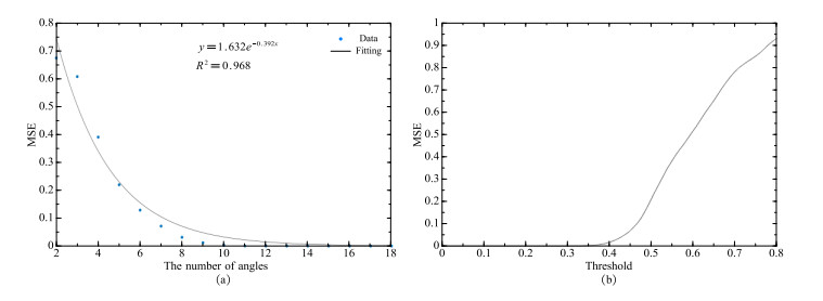
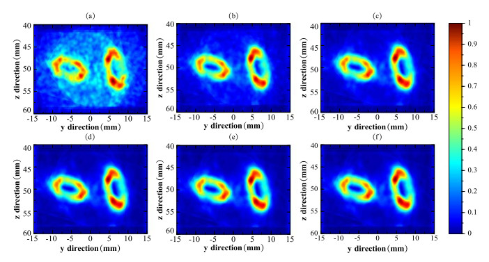
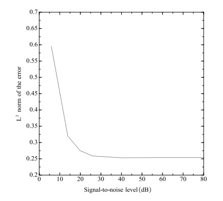
Magneto-Acousto-Electrical Tomography (MAET) is a novel multi-physics imaging method, which promises to offer a unique biophysical property of tissue electrical impedance with the additional benefit of excellent spatial resolution of the ultrasonic imaging. It opens the potential for early diagnosis of cancer by revealing changes of dielectric characteristics. However, direct MAET is unable to image the irregularly-shaped lesions fully due to the dependence on the angle between conductivity boundary and ultrasound beam direction. In this paper, a numerical simulation of multi-angle MAET is presented for an improved image reconstruction for MAET in order to discern irregularly-shaped tumors in different positions. The results show that the conductivity boundary interfaces are invisible in single angle B-mode reconstructed image, wherever the ultrasound beam and conductivity boundary are nearly parallel. When the multi-angle scanning was adopted, the image reconstructed with image rotation method reproduced the original object pattern. Furthermore, the relationship between reconstruction error and the number of angles was also discussed. It is found that 12 angles would be necessary to achieve nearly the optimal reconstruction. Finally, reconstructed images in L2 norm of the error with the measurement noise are presented.
Citation: Tong Sun, Xin Zeng, Penghui Hao, Chien Ting Chin, Mian Chen, Jiejie Yan, Ming Dai, Haoming Lin, Siping Chen, Xin Chen. Optimization of multi-angle Magneto-Acousto-Electrical Tomography (MAET) based on a numerical method[J]. Mathematical Biosciences and Engineering, 2020, 17(4): 2864-2880. doi: 10.3934/mbe.2020161
Magneto-Acousto-Electrical Tomography (MAET) is a novel multi-physics imaging method, which promises to offer a unique biophysical property of tissue electrical impedance with the additional benefit of excellent spatial resolution of the ultrasonic imaging. It opens the potential for early diagnosis of cancer by revealing changes of dielectric characteristics. However, direct MAET is unable to image the irregularly-shaped lesions fully due to the dependence on the angle between conductivity boundary and ultrasound beam direction. In this paper, a numerical simulation of multi-angle MAET is presented for an improved image reconstruction for MAET in order to discern irregularly-shaped tumors in different positions. The results show that the conductivity boundary interfaces are invisible in single angle B-mode reconstructed image, wherever the ultrasound beam and conductivity boundary are nearly parallel. When the multi-angle scanning was adopted, the image reconstructed with image rotation method reproduced the original object pattern. Furthermore, the relationship between reconstruction error and the number of angles was also discussed. It is found that 12 angles would be necessary to achieve nearly the optimal reconstruction. Finally, reconstructed images in L2 norm of the error with the measurement noise are presented.

| [1] |
D. Haemmerich, D. J. Schutt, A. W. Wright, J G Webster, D M Mahvi, Electrical conductivity measurement of excised human metastatic liver tumours before and after thermal ablation, Physiol. Meas., 30 (2009), 459-466. doi: 10.1088/0967-3334/30/5/003

|
| [2] |
A. J. Surowiec, S. S. Stuchly, J. B. Barr, A. Swarup, Dielectric properties of breast carcinoma and the surrounding tissues, IEEE Trans. Biomed. Eng., 35 (1988), 257-263. doi: 10.1109/10.1374
|
| [3] |
S. Gabriel, R. W. Lau, C. Gabriel, The dielectric properties of biological tissues: Ⅱ. Measurements in the frequency range 10 Hz to 20 GHz, Phys. Med. Biol., 41 (1996), 2251-2269. doi: 10.1088/0031-9155/41/11/002
|
| [4] |
A. Mahara, S. Khan, E. K. Murphy, A. R. Schned, E. S. Hyams, R. J. Halter, 3D microendoscopic electrical impedance tomography for margin assessment during robot-assisted laparoscopic prostatectomy, IEEE Trans. Med. Imaging, 34 (2015), 1590-1601. doi: 10.1109/TMI.2015.2407833
|
| [5] |
A. Adler, A. Boyle, Electrical impedance tomography: Tissue properties to image measures, IEEE Trans. Biomed. Eng., 64 (2017), 2494-2504. doi: 10.1109/TBME.2017.2728323
|
| [6] |
H. J. Kim, Y. T. Kim, A. S. Minhas, W. C. Jeong, E. J. Woo, J. K. Seo, et al., In vivo high-resolution conductivity imaging of the human leg using MREIT: The first human experiment, IEEE Trans. Med. Imaging, 28 (2009), 1681-1687. doi: 10.1109/TMI.2009.2018112
|
| [7] |
J. K. Seo, E. J. Woo, Electrical tissue property imaging at low frequency using MREIT, IEEE Trans. Biomed. Eng., 61 (2014), 1390-1399. doi: 10.1109/TBME.2014.2298859
|
| [8] |
Y. Kai, S. Qi, S. Ashkenazi, J. C. Bischof, H. Bin, In vivo electrical conductivity contrast imaging in a mouse model of cancer using high-frequency magnetoacoustic tomography with magnetic induction (hfMAT-MI), IEEE Trans. Med. Imaging, 35 (2016), 2301-2311. doi: 10.1109/TMI.2016.2560146
|
| [9] |
X. Li, K. Yu, B. He, Magnetoacoustic tomography with magnetic induction (MAT-MI) for imaging electrical conductivity of biological tissue: a tutorial review, Phys. Med. Biol., 61 (2016), R249-R270. doi: 10.1088/0031-9155/61/18/R249
|
| [10] |
Y. Xu, B. He, Magnetoacoustic tomography with magnetic induction (MAT-MI), Phys. Med. Biol., 50 (2005), 5175-5187. doi: 10.1088/0031-9155/50/21/015
|
| [11] |
H. Wen, J. Shah, Hall effect imaging, IEEE Trans. Biomed. Eng., 45 (1998), 119-124. doi: 10.1109/10.650364
|
| [12] |
A. Montalibet, J. Jossinet, A. Matias, Scanning electric conductivity gradients with ultrasonically-induced Lorentz force, Ultrason. Imaging, 23 (2001), 117-132. doi: 10.1177/016173460102300204
|
| [13] |
S. Haider, A. Hrbek, Y. Xu, Magneto-acousto-electrical tomography: A potential method for imaging current density and electrical impedance, Physiol. Meas., 29 (2008), S41-S50. doi: 10.1088/0967-3334/29/6/S04
|
| [14] |
P. Grasland-Mongrain, J. M. Mari, J. Y. Chapelon, C. Lafon, Lorentz force electrical impedance tomography, Irbm, 34 (2013), 357-360. doi: 10.1016/j.irbm.2013.08.002
|
| [15] |
P. Graslandmongrain, F. Destrempes, J. M. Mari, R. Souchon, S. Catheline, J. Y. Chapelon, et al., Acousto-electrical speckle pattern in Lorentz force electrical impedance tomography, Phys. Med. Biol., 60 (2015), 3747-3757. doi: 10.1088/0031-9155/60/9/3747
|
| [16] |
Z. Sun, G. Liu, H. Xia, S. Catheline, Lorentz force electrical-impedance tomography using linearly frequency-modulated ultrasound pulse, IEEE Trans. Ultrason. Ferroelectr. Freq. Control, 65 (2018), 168-177. doi: 10.1109/TUFFC.2017.2781189
|
| [17] |
L. Kunyansky, C. P. Ingram, R. S. Witte, Rotational magneto-acousto-electric tomography (MAET): Theory and experimental validation, Phys. Med. Biol., 62 (2017), 3025-3050. doi: 10.1088/1361-6560/aa6222
|
| [18] |
A. Montalibet, J. Jossinet, A. Matias, D. Cathignol, Electric current generated by ultrasonically induced Lorentz force in biological media, Med. Biol. Eng. Comput., 39 (2001), 15-20. doi: 10.1007/BF02345261
|
| [19] | A. G. Stove, Linear FMCW radar techniques, Radar Signal Process. Iee Process. F, 139 (1992), 343-350. |
| [20] |
M. Dai, X. Chen, T. Sun, L. Yu, A 2D Magneto-Acousto-Electrical Tomography method to detect conductivity variation using multifocus image method, Sensors, 18 (2018), 2373-2388. doi: 10.3390/s18072373
|
| [21] |
M. Dai, T. Sun, X. Chen, L. Yu, M. Chen, P. Hao, A B-scan imaging method of conductivity variation detection for Magneto-Acousto-Electrical Tomography, IEEE Access, 7 (2019), 26881-26891. doi: 10.1109/ACCESS.2019.2899164
|
| [22] |
R. Zengin, N. G. Gencer, Lorentz force electrical impedance tomography using magnetic field measurements, Phys. Med. Biol., 61 (2016), 5887-5905. doi: 10.1088/0031-9155/61/16/5887
|
| [23] |
M. S. GöZü, R. Zengin, N. G. Gencer, Numerical implementation of magneto-acousto-electric tomography (MAET) using a linear phased array transducer, Phys. Med. Biol., 63 (2018), 035012. doi: 10.1088/1361-6560/aa9f3b
|
| [24] |
B. Cockburn, C. W. Shu, Runge-Kutta discontinuous galerkin methods for convection-dominated problems, J. Sci. Comput., 16 (2001), 173-261. doi: 10.1023/A:1012873910884
|
| [25] |
N. Polydorides, Finite element modelling and image reconstruction for Lorentz force electrical impedance tomography, Physiol. Meas., 39 (2018), 44003. doi: 10.1088/1361-6579/aab657
|
| [26] |
C. Gabriel, S. Gabriel, E. Corthout, The dielectric properties of biological tissues: Ⅰ. Literature survey, Phys. Med. Biol., 41 (1996), 2231-2249. doi: 10.1088/0031-9155/41/11/001
|
| [27] |
S. Gabriel, R. W. Lau, C. Gabriel, The dielectric properties of biological tissues: Ⅲ. Parametric models for the dielectric spectrum of tissues, Phys. Med. Biol., 41 (1996), 2271-2293. doi: 10.1088/0031-9155/41/11/003
|
Figures(15) / Tables(2)

Tong Sun, Xin Zeng, Penghui Hao, Chien Ting Chin, Mian Chen, Jiejie Yan, Ming Dai, Haoming Lin, Siping Chen, Xin Chen. Optimization of multi-angle Magneto-Acousto-Electrical Tomography (MAET) based on a numerical method[J]. Mathematical Biosciences and Engineering, 2020, 17(4): 2864-2880. doi: 10.3934/mbe.2020161


 DownLoad: