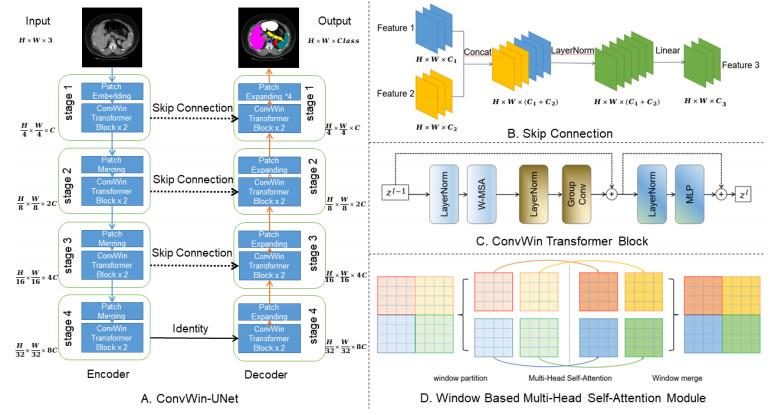
Convolutional Neural Network (CNN) plays a vital role in the development of computer vision applications. The depth neural network composed of U-shaped structures and jump connections is widely used in various medical image tasks. Recently, based on the self-attention mechanism, the Transformer structure has made great progress and tends to replace CNN, and it has great advantages in understanding global information. In this paper, the ConvWin Transformer structure is proposed, which refers to the W-MSA structure in Swin and combines with the convolution. It can not only accelerate the convergence speed, but also enrich the information exchange between patches and improve the understanding of local information. Then, it is integrated with UNet, a U-shaped architecture commonly used in medical image segmentation, to form a structure called ConvWin-UNet. Meanwhile, this paper improves the patch expanding layer to perform the upsampling operation. The experimental results on the Hubmap datasets and synapse multi-organ segmentation dataset indicate that the proposed ConvWin-UNet structure achieves excellent results. Partial code and models of this work are available at https://github.com/xmFeng-hdu/ConvWin-UNet.
Citation: Xiaomeng Feng, Taiping Wang, Xiaohang Yang, Minfei Zhang, Wanpeng Guo, Weina Wang. ConvWin-UNet: UNet-like hierarchical vision Transformer combined with convolution for medical image segmentation[J]. Mathematical Biosciences and Engineering, 2023, 20(1): 128-144. doi: 10.3934/mbe.2023007
Convolutional Neural Network (CNN) plays a vital role in the development of computer vision applications. The depth neural network composed of U-shaped structures and jump connections is widely used in various medical image tasks. Recently, based on the self-attention mechanism, the Transformer structure has made great progress and tends to replace CNN, and it has great advantages in understanding global information. In this paper, the ConvWin Transformer structure is proposed, which refers to the W-MSA structure in Swin and combines with the convolution. It can not only accelerate the convergence speed, but also enrich the information exchange between patches and improve the understanding of local information. Then, it is integrated with UNet, a U-shaped architecture commonly used in medical image segmentation, to form a structure called ConvWin-UNet. Meanwhile, this paper improves the patch expanding layer to perform the upsampling operation. The experimental results on the Hubmap datasets and synapse multi-organ segmentation dataset indicate that the proposed ConvWin-UNet structure achieves excellent results. Partial code and models of this work are available at https://github.com/xmFeng-hdu/ConvWin-UNet.

| [1] | O. Ronneberger, P. Fischer, T. Brox, U-Net: convolutional networks for biomedical image segmentation, in International Conference on Medical Image Computing and Computer-Assisted Intervention, (2015), 234–241. Available from: https://link.springer.com/chapter/10.1007/978-3-319-24574-4_28. |
| [2] |
Z. Zhou, M. Siddiquee, N. Tajbakhsh, J. Liang, UNet++: redesigning skip connections to exploit multiscale features in image segmentation, IEEE Trans. Med. Imaging, 39 (2020), 1856–1867. https://doi.org/10.1109/TMI.2019.2959609 doi: 10.1109/TMI.2019.2959609

|
| [3] | H. Huang, L. Lin, R. Tong, H. Hu, Q. Zhang, Y. Iwamoto, et al., Unet 3+: a full-scale connected UNet for medical image segmentation, in ICASSP 2020 - 2020 IEEE International Conference on Acoustics, Speech and Signal Processing (ICASSP), (2020), 1055–1059. https://doi.org/10.1109/ICASSP40776.2020.9053405 |
| [4] |
X. Qin, Z. Zhang, C. Huang, M. Dehghan, O. R. Zaiane, M. Jagersand, U$^2$-Net: going deeper with nested U-structure for salient object detection, Pattern Recognit., 106 (2020), 107404. https://doi.org/10.1016/j.patcog.2020.107404 doi: 10.1016/j.patcog.2020.107404
|
| [5] | F. Isensee, P. F. Jaeger, S. A. Kohl, J. Petersen, K. H. Maier-Hein, nnU-Net: a self-configuring method for deep learning-based biomedical image segmentation, Nat. Methods, 18 (2021), 203–211. Available from: https://www.nature.com/articles/s41592-020-01008-z. |
| [6] | Q. Jin, Z. Meng, C. Sun, H. Cui, R. Su, RA-UNet: a hybrid deep attention-aware network to extra liver and tumor in ct scans, preprint, arXiv: 1811.01328. |
| [7] | Ö, Çiçek, A. Abdulkadir, S. S. Lienkamp, T. Brox, O. Ronneberger, 3D U-Net: learning dense volumetric segmentation from sparse annotation, in International Conference on Medical Image Computing and Computer-Assisted Intervention, (2016), 424–432. Available from: https://link.springer.com/chapter/10.1007/978-3-319-46723-8_49. |
| [8] | X. Xiao, S. Lian, Z. Luo, S. Li, Weighted res-unet for high-quality retina vessel segmentation, in 2018 9th International Conference on Information Technology in Medicine and Education (ITME), (2018), 327–331. https://doi.org/10.1109/ITME.2018.00080 |
| [9] |
G. Rani, P. Thakkar, A. Verma, V. Mehta, R. Chavan, V. S. Dhaka, et al., KUB-UNet: segmentation of organs of urinary system from a KUB X-ray image, Comput. Methods Programs Biomed., 224 (2022), 107031. https://doi.org/10.1016/j.cmpb.2022.107031 doi: 10.1016/j.cmpb.2022.107031
|
| [10] | A. Vaswani, N. Shazeer, N. Parmar, J. Uszkoreit, L. Jones, A. N. Gomez, et al., Attention is all you need, in Advances in Neural Information Processing Systems, (2017), 5998–6008. https://doi.org/10.48550/arXiv.1706.03762 |
| [11] | A. Dosovitskiy, L. Beyer, A. Kolesnikov, D. Weissenborn, X. Zhai, T. Unterthiner, et al., An image is worth 16x16 words: transformers for image recognition at scale, preprint, arXiv: 2010.11929. |
| [12] | J. Chen, Y. Lu, Q. Yu, X. Luo, E. Adeli, Y. Wang, et al., Transunet: transformers make strong encoders for medical image segmentation, preprint, arXiv: 2102.04306. |
| [13] | H. Cao, Y. Wang, J. Chen, D. Jiang, X. Zhang, Q. Tian, et al., Swin-Unet: Unet-like pure transformer for medical image segmentation, preprint, arXiv: 2105.05537. |
| [14] | C. Yao, M. Hu, G. Zhai, X. P. Zhang, Transclaw U-Net: claw U-Net with transformers for medical image segmentation, preprint, arXiv: 2107.05188. |
| [15] | H. Wang, S. Xie, L. Lin, Y. Iwamoto, X. Han, Y. Chen, et al., Mixed transformer u-net for medical image segmentation, in International Conference on Acoustics, Speech and Signal Processing (ICASSP), (2022), 2390–2394. Available from: https://ieeexplore.ieee.org/abstract/document/9746172. |
| [16] | H. Touvron, M. Cord, M. Douze, F. Massa, A. Sablayrolles, H. Jégou, Training data-efficient image transformers & distillation through attention, preprint, arXiv: 2012.12877. |
| [17] | Z. Liu, Y. Lin, Y. Cao, H. Hu, Y. Wei, Z. Zhang, et al., Swin transformer: hierarchical vision transformer using shifted windows, preprint, arXiv: 2103.14030. |
| [18] | Synapse multi-organ segmentation dataset. Available from: https://www.synapse.org/#!Synapse:syn3193805/wiki/217789. |
| [19] | HuBMAP - Hacking the Kidney Identify glomeruli in human kidney tissue images. Available from: https://www.kaggle.com/c/hubmap-kidney-segmentation/data. |
| [20] |
A. Krizhevsky, I. Sutskever, G. E. Hinton, ImageNet classification with deep convolutional neural networks, Commun. ACM, 60 (2017), 84–90. https://doi.org/10.1145/3065386 doi: 10.1145/3065386
|
| [21] | K. Simonyan, A. Zisserman, Very deep convolutional networks for large-scale image recognition, preprint, arXiv: 1409.1556 |
| [22] | C. Szegedy, W. Liu, Y. Jia, P. Sermanet, S. Reed, D. Anguelov, et al., Going deeper with convolutions, in 2015 IEEE Conference on Computer Vision and Pattern Recognition (CVPR), (2015), 1–9. https://doi.org/10.1109/CVPR.2015.7298594 |
| [23] | K. He, X. Zhang, S. Ren, J. Sun, Deep residual learning for image recognition, in 2016 IEEE Conference on Computer Vision and Pattern Recognition (CVPR), (2016), 770–778. https://doi.org/10.1109/CVPR.2016.90 |
| [24] | G. Huang, Z. Liu, L. Van Der Maaten, K. Q. Weinberger, Densely connected convolutional networks, preprint, arXiv: 1608.06993. |
| [25] | M. Tan, Q. Le, Efficientnet: rethinking model scaling for convolutional neural networks, preprint, arXiv: 1905.11946. |
| [26] | P. T. De Boer, D. P. Kroese, S. Mannor, R. Y. Rubinstein, A tutorial on the cross-entropy method, Ann. Oper. Res., 134 (2005), 19–67. Available from: https://link.springer.com/article/10.1007/s10479-005-5724-z. |
| [27] | F. Milletari, N. Navab, S. A. Ahmadi, V-net: fully convolutional neural networks for volumetric medical image segmentation, in 2016 Fourth International Conference on 3D Vision (3DV), (2016), 565–571. https://doi.org/10.1109/3DV.2016.79 |
| [28] |
Z. Wang, A. C. Bovik, H. R. Sheikh, E. P. Simoncelli, Image quality assessment: from error visibility to structural similarity, IEEE Trans. Image Process., 13 (2004), 600–612. https://doi.org/10.1109/TIP.2003.819861 doi: 10.1109/TIP.2003.819861
|
| [29] | Z. Wang, E. P. Simoncelli, A. C. Bovik, Multiscale structural similarity for image quality assessment, in The Thrity-Seventh Asilomar Conference on Signals, Systems Computers, 2003, (2003), 1398–1402. https://doi.org/10.1109/ACSSC.2003.1292216 |
| [30] | S. Fu, Y. Lu, Y. Wang, Y. Zhou, W. Shen, E. Fishman, et al., Domain adaptive relational reasoning for 3d multi-organ segmentation, preprint, arXiv: 2005.09120. |
| [31] | O. Oktay, J. Schlemper, L. L. Folgoc, M. Lee, M. Heinrich, K. Misawa, et al., Attention u-net: learning where to look for the pancreas, preprint, arXiv: 1804.03999v3. |
Figures(8) / Tables(5)

Xiaomeng Feng, Taiping Wang, Xiaohang Yang, Minfei Zhang, Wanpeng Guo, Weina Wang. ConvWin-UNet: UNet-like hierarchical vision Transformer combined with convolution for medical image segmentation[J]. Mathematical Biosciences and Engineering, 2023, 20(1): 128-144. doi: 10.3934/mbe.2023007


 DownLoad: