Path planning and collision avoidance methods for distributed multi-robot systems in complex dynamic environments

Zhen Yang; Junli Li; Liwei Yang; Qian Wang; Ping Li; Guofeng Xia; Zhen Yang; Junli Li; Liwei Yang; Qian Wang; Ping Li; Guofeng Xia

doi:10.3934/mbe.2023008

Mathematical Biosciences and Engineering

2023, Volume 20, Issue 1: 145-178. doi: 10.3934/mbe.2023008

Previous Article Next Article

Research article Special Issues

Path planning and collision avoidance methods for distributed multi-robot systems in complex dynamic environments

School of Information Engineering and Automation, Kunming University of Science and Technology, Kunming 650093, China

Academic Editor: Ping Jiang

Received: 01 June 2022 Revised: 10 August 2022 Accepted: 25 August 2022 Published: 30 September 2022

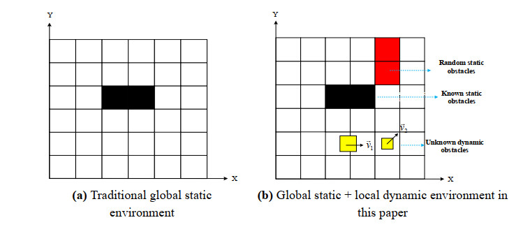
Multi-robot systems are experiencing increasing popularity in joint rescue, intelligent transportation, and other fields. However, path planning and navigation obstacle avoidance among multiple robots, as well as dynamic environments, raise significant challenges. We propose a distributed multi-mobile robot navigation and obstacle avoidance method in unknown environments. First, we propose a bidirectional alternating jump point search A* algorithm (BAJPSA*) to obtain the robot's global path in the prior environment and further improve the heuristic function to enhance efficiency. We construct a robot kinematic model based on the dynamic window approach (DWA), present an adaptive navigation strategy, and introduce a new path tracking evaluation function that improves path tracking accuracy and optimality. To strengthen the security of obstacle avoidance, we modify the decision rules and obstacle avoidance rules of the single robot and further improve the decision avoidance capability of multi-robot systems. Moreover, the mainstream prioritization method is used to coordinate the local dynamic path planning of our multi-robot systems to resolve collision conflicts, reducing the difficulty of obstacle avoidance and simplifying the algorithm. Experimental results show that this distributed multi-mobile robot motion planning method can provide better navigation and obstacle avoidance strategies in complex dynamic environments, which provides a technical reference in practical situations.
- distributed multi-mobile robots,
- path planning,
- A* algorithm,
- dynamic window approach,
- prioritization method
Citation: Zhen Yang, Junli Li, Liwei Yang, Qian Wang, Ping Li, Guofeng Xia. Path planning and collision avoidance methods for distributed multi-robot systems in complex dynamic environments[J]. Mathematical Biosciences and Engineering, 2023, 20(1): 145-178. doi: 10.3934/mbe.2023008

Related Papers:

Abstract

Multi-robot systems are experiencing increasing popularity in joint rescue, intelligent transportation, and other fields. However, path planning and navigation obstacle avoidance among multiple robots, as well as dynamic environments, raise significant challenges. We propose a distributed multi-mobile robot navigation and obstacle avoidance method in unknown environments. First, we propose a bidirectional alternating jump point search A* algorithm (BAJPSA*) to obtain the robot's global path in the prior environment and further improve the heuristic function to enhance efficiency. We construct a robot kinematic model based on the dynamic window approach (DWA), present an adaptive navigation strategy, and introduce a new path tracking evaluation function that improves path tracking accuracy and optimality. To strengthen the security of obstacle avoidance, we modify the decision rules and obstacle avoidance rules of the single robot and further improve the decision avoidance capability of multi-robot systems. Moreover, the mainstream prioritization method is used to coordinate the local dynamic path planning of our multi-robot systems to resolve collision conflicts, reducing the difficulty of obstacle avoidance and simplifying the algorithm. Experimental results show that this distributed multi-mobile robot motion planning method can provide better navigation and obstacle avoidance strategies in complex dynamic environments, which provides a technical reference in practical situations.

References

[1]	F. Rubio, F. Valero, C. Llopis-Albert, A review of mobile robots: Concepts, methods, theoretical framework, and applications, Int. J. Adv. Rob.Syst., 16 (2019), 1729881419839596. https://doi.org/10.1177/1729881419839596 doi: 10.1177/1729881419839596
[2]	S. J. Fusic, G. Kanagaraj, K. Hariharan, S. Karthikeyan, Optimal path planning of autonomous navigation in outdoor environment via heuristic technique, Transp. Res. Interdiscip. Perspect., 12 (2021), 100473. https://doi.org/10.1016/j.trip.2021.100473 doi: 10.1016/j.trip.2021.100473
[3]	J. Li, J. Sun, L. Liu, J. Xu, Model predictive control for the tracking of autonomous mobile robot combined with a local path planning, Meas. Control, 54 (2021), 1319–1325. https://doi.org/10.1177/00202940211043070 doi: 10.1177/00202940211043070
[4]	A. V. Le, V. Prabakaran, V. Sivanantham, R. E. Mohan, Modified a-star algorithm for efficient coverage path planning in tetris inspired self-reconfigurable robot with integrated laser sensor, Sensors, 18 (2018), 2585. https://doi.org/10.3390/s18082585 doi: 10.3390/s18082585
[5]	H. Wang, X. Qi, S. Lou, J. Jing, H. He, W. Liu, An efficient and robust improved A* algorithm for path planning, Symmetry, 13 (2021), 2213. https://doi.org/10.3390/sym13112213 doi: 10.3390/sym13112213
[6]	B. Zhang, D. Zhu, A new method on motion planning for mobile robots using jump point search and Bezier curves, Int. J. Adv. Robot. Syst., 18 (2021), 17298814211019220. https://doi.org/10.1177/17298814211019220 doi: 10.1177/17298814211019220
[7]	F. H. Ajeil, I. Ibraheem, A. T. Azar, A. J. Humaidi, Grid-based mobile robot path planning using aging-based ant colony optimization algorithm in static and dynamic environments, Sensors, 20 (2020), 1880. https://doi.org/10.3390/s20071880 doi: 10.3390/s20071880
[8]	C. Miao, G. Chen, C. Yan, Y. Wu, Path planning optimization of indoor mobile robot based on adaptive ant colony algorithm, Comput. Indust. Eng., 156 (2021), 107230. https://doi.org/10.1016/j.cie.2021.107230 doi: 10.1016/j.cie.2021.107230
[9]	B. Song, Z. Wang, L. Zou, An improved PSO algorithm for smooth path planning of mobile robots using continuous high-degree Bezier curve, Appl. Soft Comput., 100 (2021), 106960. https://doi.org/10.1016/j.asoc.2020.106960 doi: 10.1016/j.asoc.2020.106960
[10]	X. Guo, M. Ji, Z. Zhao, W. Zhang, Global path planning and multi-objective path control for unmanned surface vehicle based on modified particle swarm optimization (PSO) algorithm, Ocean Eng., 216 (2020), 107693. https://doi.org/10.1016/j.oceaneng.2020.107693 doi: 10.1016/j.oceaneng.2020.107693
[11]	M. A. Hossain, I. Ferdous, Autonomous robot path planning in dynamic environment using a new optimization technique inspired by bacterial foraging technique, Robot. Auton. Syst., 64 (2015), 137–141. https://doi.org/10.1016/j.robot.2014.07.002 doi: 10.1016/j.robot.2014.07.002
[12]	Y. P. Chen, Y. Li, G. Wang, Y. F. Zheng, Q. Xu, J. H. Fan, et al., A novel bacterial foraging optimization algorithm for feature selection, Expert Syst. Appl., 83 (2017), 1–17. https://doi.org/10.1016/j.eswa.2017.04.019 doi: 10.1016/j.eswa.2017.04.019
[13]	H. Tang, W. Sun, H. Yu, A. Lin, M. Xue, A multirobot target searching method based on bat algorithm in unknown environments, Expert Syst. Appl., 141 (2020), 112945. https://doi.org/10.1016/j.eswa.2019.112945 doi: 10.1016/j.eswa.2019.112945
[14]	G. G. Wang, H. E. Chu, S. Mirjalili, Three-dimensional path planning for UCAV using an improved bat algorithm, Aerosp. Sci. Technol., 49 (2016), 231–238. https://doi.org/10.1016/j.ast.2015.11.040 doi: 10.1016/j.ast.2015.11.040
[15]	Z. Yan, J. Zhang, J. Zeng, J. Tang, Three-dimensional path planning for autonomous underwater vehicles based on a whale optimization algorithm, Ocean Eng., 250 (2022), 111070. https://doi.org/10.1016/j.oceaneng.2022.111070 doi: 10.1016/j.oceaneng.2022.111070
[16]	F. Gul, I. Mir, L. Abualigah, S. Mir, M. Altalhi, Cooperative multi-function approach: A new strategy for autonomous ground robotics, Future Gener. Comput. Syst., 134 (2022), 361–373. https://doi.org/10.1016/j.future.2022.04.007 doi: 10.1016/j.future.2022.04.007
[17]	D. Foead, A. Ghifari, M. B. Kusuma, N. Hanafiah, E. Gunawan, A systematic literature review of A* pathfinding, Proc. Comput. Sci., 179 (2021), 507–514. https://doi.org/10.1016/j.procs.2021.01.034 doi: 10.1016/j.procs.2021.01.034
[18]	Q. Wu, Z. Chen, L. Wang, H. Lin, Z. Jiang, S. Li, et al., Real-time dynamic path planning of mobile robots: A novel hybrid heuristic optimization algorithm, Sensors, 20 (2020), 188. https://doi.org/10.3390/s20010188 doi: 10.3390/s20010188
[19]	L. Chang, L. Shan, Y. Dai, Multi-robot formation control in unknown environment based on improved DWA, Control Decis., (2021), 1–10. https://doi.org/10.13195/j.kzyjc.2020.1817. doi: 10.13195/j.kzyjc.2020.1817
[20]	J. Sun, G. Liu, G. Tian, J. Zhang, Smart obstacle avoidance using a danger index for a dynamic environment, Appl. Sci., 9 (2019), 1589. https://doi.org/10.3390/app9081589 doi: 10.3390/app9081589
[21]	L. Chang, L. Shan, C. Jiang, Y. Dai, Reinforcement based mobile robot path planning with improved dynamic window approach in unknown environment, Auton. Robot., 45 (2021), 51–76. https://doi.org/10.1007/s10514-020-09947-4 doi: 10.1007/s10514-020-09947-4
[22]	Z. Lin, M. Yue, G. Chen, J. Sun, Path planning of mobile robot with PSO-based APF and fuzzy-based DWA subject to moving obstacles, Trans. Inst. Meas. Control, 44 (2022), 121–132. https://doi.org/10.1177/01423312211024798 doi: 10.1177/01423312211024798
[23]	Y. Chen, G. Luo, Y. Mei, J. Yu, X. Su, UAV path planning using artificial potential field method updated by optimal control theory, Int. J. Syst. Sci., 47 (2016), 1407–1420. https://doi.org/10.1080/00207721.2014.929191 doi: 10.1080/00207721.2014.929191
[24]	U. Orozco-Rosas, O. Montiel, R. Sepúlveda, Mobile robot path planning using membrane evolutionary artificial potential field, Appl. Soft Comput., 77 (2019), 236–251. https://doi.org/10.1016/j.asoc.2019.01.036 doi: 10.1016/j.asoc.2019.01.036
[25]	X. Zhong, J. Tian, H. Hu, X. Peng, Hybrid path planning based on safe A* algorithm and adaptive window approach for mobile robot in large-scale dynamic environment, J. Intell. Robot. Syst., 99 (2020), 65–77. https://doi.org/10.1007/s10846-019-01112-z doi: 10.1007/s10846-019-01112-z
[26]	X. Ji, S. Feng, Q. Han, H. Yin, S. Yu, Improvement and fusion of A* algorithm and dynamic window approach considering complex environmental information, Arab. J. Sci. Eng., 46 (2021), 7445–7459. https://doi.org/10.1007/s13369-021-05445-6 doi: 10.1007/s13369-021-05445-6
[27]	Z. Wang, G. Li, J. Ren, Dynamic path planning for unmanned surface vehicle in complex offshore areas based on hybrid algorithm, Comput. Commun., 166 (2021), 49–56. https://doi.org/10.1016/j.comcom.2020.11.012 doi: 10.1016/j.comcom.2020.11.012
[28]	B. Sahu, P. K. Das, M. Kabat, Multi-robot cooperation and path planning for stick transporting using improved Q-learning and democratic robotics PSO, J. Comput. Sci., 60 (2022), 101637. https://doi.org/10.1016/j.jocs.2022.101637 doi: 10.1016/j.jocs.2022.101637
[29]	Y. Dai, Y. Kim, S. Wee, D. Lee, S. Lee, A switching formation strategy for obstacle avoidance of a multi-robot system based on robot priority model, ISA Trans., 56 (2015), 123–134. https://doi.org/10.1016/j.isatra.2014.10.008 doi: 10.1016/j.isatra.2014.10.008
[30]	H. Sang, Y. You, X. Sun, Y. Zhou, F. Liu, The hybrid path planning algorithm based on improved A* and artificial potential field for unmanned surface vehicle formations, Ocean Eng., 23 (2021), 108709. https://doi.org/10.1016/j.oceaneng.2021.108709 doi: 10.1016/j.oceaneng.2021.108709
[31]	P. K. Das, H. S. Behera, B. K. Panigrahi, A hybridization of an improved particle swarm optimization and gravitational search algorithm for multi-robot path planning, Swarm Evol. Comput., 28 (2016), 14–28. https://doi.org/10.1016/j.swevo.2015.10.011 doi: 10.1016/j.swevo.2015.10.011
[32]	P. K. Das, P. K. Jena, Multi-robot path planning using improved particle swarm optimization algorithm through novel evolutionary operators, Appl. Soft Comput., 92 (2020), 106312. https://doi.org/10.1016/j.asoc.2020.106312 doi: 10.1016/j.asoc.2020.106312
[33]	R. K. Dewangan, A. Shukla, W. W. Godfrey, A solution for priority-based multi-robot path planning problem with obstacles using ant lion optimization, Mod. Phys. Lett. B, 34 (2020), 2050137. https://doi.org/10.1142/S0217984920501377 doi: 10.1142/S0217984920501377
[34]	J. M. Yang, C. M. Tseng, P. S. Tseng, Path planning on satellite images for unmanned surface vehicles, Int. J. Naval Archit. Ocean Eng., 7 (2015), 87–99. https://doi.org/10.1515/ijnaoe-2015-0007 doi: 10.1515/ijnaoe-2015-0007
[35]	L. Yang, L. Fu, P. Li, J. Mao, N. Guo, L. Du, LF-ACO: An effective formation path planning for multi-mobile robot, Math. Biosci. Eng., 19 (2022), 225–252. https://doi.org/10.3934/mbe.2022012 doi: 10.3934/mbe.2022012
[36]	D. Harabor, A. Grastien, Online graph pruning for pathfinding on grid maps, in Proceedings of the AAAI Conference on Artificial Intelligence, 25 (2011), 1114–1119. https://doi.org/10.1609/aaai.v25i1.7994
[37]	D. Harabor, A. Grastien, Improving jump point search, in Proceedings of the International Conference on Automated Planning and Scheduling, 24 (2014), 128–135.
[38]	C. Li, X. Huang, J. Ding, K. Song, S. Lu, Global path planning based on a bidirectional alternating search A* algorithm for mobile robots, Comput. Indust. Eng., 168 (2022), 108123. https://doi.org/10.1016/j.cie.2022.108123 doi: 10.1016/j.cie.2022.108123
[39]	Y. Singh, S. Sharma, R. Sutton, D. Hatton, A. Khan, A constrained A* approach towards optimal path planning for an unmanned surface vehicle in a maritime environment containing dynamic obstacles and ocean currents, Ocean Eng., 169 (2018), 187–201. https://doi.org/10.1016/j.oceaneng.2018.09.016 doi: 10.1016/j.oceaneng.2018.09.016
[40]	L. Yang, L. Fu, P. Li, J. Mao, N. Guo, An effective dynamic path planning approach for mobile robots based on ant colony fusion dynamic windows, Machines, 10 (2022), 50. https://doi.org/10.3390/machines10010050 doi: 10.3390/machines10010050
[41]	S. M. H. Rostami, A. K. Sangaiah, J. Wang, X. Liu, Obstacle avoidance of mobile robots using modified artificial potential field algorithm, EURASIP J. Wirel. Commun. Netw., 2019 (2019), 1–19. https://doi.org/10.1186/s13638-019-1396-2 doi: 10.1186/s13638-019-1396-2
[42]	E. A. Torkamani, Z. Xi, Systematical collision avoidance reliability analysis and characterization of reliable system operation for autonomous navigation using the dynamic window approach, ASCE-ASME J. Risk Uncertainty Eng. Syst., Part B, 8 (2022), 031106. https://doi.org/10.1115/1.4053941 doi: 10.1115/1.4053941
[43]	C. Liang, X. Zhang, Y. Watanabe, Y. Deng, Autonomous collision avoidance of unmanned surface vehicles based on improved A star and minimum course alteration algorithms, Appl. Ocean Res., 113 (2021), 102755. https://doi.org/10.1016/j.apor.2021.102755 doi: 10.1016/j.apor.2021.102755
[44]	M. Kobayashi, N. Motoi, Local path planning: Dynamic window approach with virtual manipulators considering dynamic obstacles, IEEE Access, 10 (2022), 17018–17029. https://doi.org/10.1109/ACCESS.2022.3150036 doi: 10.1109/ACCESS.2022.3150036
[45]	E. Olcay, F. Schuhmann, B. Lohmann, Collective navigation of a multi-robot system in an unknown environment, Robot. Auton. Syst., 132 (2020), 103604. https://doi.org/10.1016/j.robot.2020.103604 doi: 10.1016/j.robot.2020.103604
[46]	L. Gracia, A. Sala, F. Garelli, Robot coordination using task-priority and sliding-mode techniques, Robot. Comput. Integr. Manuf., 30 (2024), 74–89. https://doi.org/10.1016/j.rcim.2013.08.003 doi: 10.1016/j.rcim.2013.08.003

Reader Comments

Your name:*

Email:*
© 2023 the Author(s), licensee AIMS Press. This is an open access article distributed under the terms of the Creative Commons Attribution License (http://creativecommons.org/licenses/by/4.0)