Habitat loss and fragmentation is the largest contributing factor to species extinction and declining biodiversity. Landscapes are becoming highly spatially heterogeneous with varying degrees of human modification. Much theoretical study of habitat fragmentation has historically focused on a simple theoretical landscape with patches of habitat surrounded by a spatially homogeneous hostile matrix. However, terrestrial habitat patches are often surrounded by complex mosaics of many different land cover types, which are rarely ecologically neutral or completely inhospitable environments. We employ an extension of a reaction diffusion model to explore effects of heterogeneity in the matrix immediately surrounding a patch in a one-dimensional theoretical landscape. Exact dynamics of a population exhibiting logistic growth, an unbiased random walk in the patch and matrix, habitat preference at the patch/matrix interface, and two functionally different matrix types for the one-dimensional landscape is obtained. These results show existence of a minimum patch size (MPS), below which population persistence is not possible. This MPS can be estimated via empirically derived estimates of patch intrinsic growth rate and diffusion rate, habitat preference, and matrix death and diffusion rates. We conclude that local matrix heterogeneity can greatly change model predictions, and argue that conservation strategies should not only consider patch size, configuration, and quality, but also quality and spatial structure of the surrounding matrix.
Citation: Nalin Fonseka, Jerome Goddard Ⅱ, Alketa Henderson, Dustin Nichols, Ratnasingham Shivaji. Modeling effects of matrix heterogeneity on population persistence at the patch-level[J]. Mathematical Biosciences and Engineering, 2022, 19(12): 13675-13709. doi: 10.3934/mbe.2022638
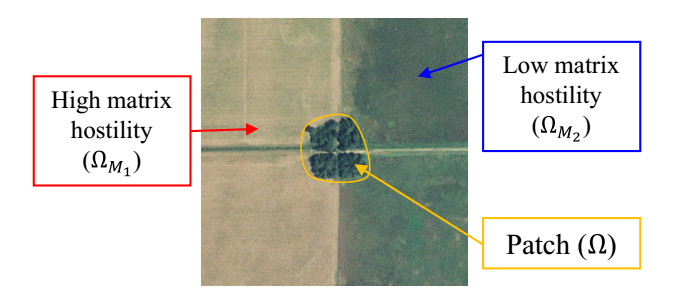
Habitat loss and fragmentation is the largest contributing factor to species extinction and declining biodiversity. Landscapes are becoming highly spatially heterogeneous with varying degrees of human modification. Much theoretical study of habitat fragmentation has historically focused on a simple theoretical landscape with patches of habitat surrounded by a spatially homogeneous hostile matrix. However, terrestrial habitat patches are often surrounded by complex mosaics of many different land cover types, which are rarely ecologically neutral or completely inhospitable environments. We employ an extension of a reaction diffusion model to explore effects of heterogeneity in the matrix immediately surrounding a patch in a one-dimensional theoretical landscape. Exact dynamics of a population exhibiting logistic growth, an unbiased random walk in the patch and matrix, habitat preference at the patch/matrix interface, and two functionally different matrix types for the one-dimensional landscape is obtained. These results show existence of a minimum patch size (MPS), below which population persistence is not possible. This MPS can be estimated via empirically derived estimates of patch intrinsic growth rate and diffusion rate, habitat preference, and matrix death and diffusion rates. We conclude that local matrix heterogeneity can greatly change model predictions, and argue that conservation strategies should not only consider patch size, configuration, and quality, but also quality and spatial structure of the surrounding matrix.

| [1] | E. O. Wilson, Threats to biodiversity, Sci. Am., 261 (1989), 108–117. http://www.jstor.org/stable/24987402 |
| [2] |
L. Fahrig, How much habitat is enough?, Biol. Conserv., 100 (2001), 65–74. https://doi.org/10.1016/S0006-3207(00)00208-1 doi: 10.1016/S0006-3207(00)00208-1

|
| [3] |
I. Hanski, Habitat loss, the dynamics of biodiversity, and a perspective on conservation, AMBIO, 40 (2011), 248–255. https://doi.org/10.1007/s13280-011-0147-3 doi: 10.1007/s13280-011-0147-3
|
| [4] |
D. Tilman, M. Clark, D. R. Williams, K. Kimmel, S. Polasky, C. Packer, Future threats to biodiversity and pathways to their prevention, Nature, 546 (2017), 73–81. https://doi.org/10.1038/nature22900 doi: 10.1038/nature22900
|
| [5] |
K. J. J. Kuipers, J. P. Hilbers, J. Garcia-Ulloa, B. J. Graae, R. May, F. Verones, et al., Habitat fragmentation amplifies threats from habitat loss to mammal diversity across the world's terrestrial ecoregions, One Earth, 4 (2021), 1505–1513. https://doi.org/10.1016/j.oneear.2021.09.005 doi: 10.1016/j.oneear.2021.09.005
|
| [6] | J. F. Brodie, W. D. Newmark, Heterogeneous matrix habitat drives species occurrences in complex, fragmented landscapes, Am. Nat., 193 (2019), 748–754. https://www.journals.uchicago.edu/doi/abs/10.1086/702589 |
| [7] |
M. A. Bowers, S. F. Matter, Landscape ecology of mammals: Relationships between density and patch size, J. Mammal., 78 (1997), 999–1013. https://doi.org/10.2307/1383044 doi: 10.2307/1383044
|
| [8] |
D. J. Bender, T. A. Contreras, L. Fahrig, Habitat loss and population decline: A meta-analysis of the patch size effect, Ecology, 79 (1998), 517–533. https://doi.org/10.1890/0012-9658(1998)079[0517:HLAPDA]2.0.CO;2 doi: 10.1890/0012-9658(1998)079[0517:HLAPDA]2.0.CO;2
|
| [9] |
E. F. Connor, A. C. Courtney, J. M. Yoder, Individuals–area relationships: The relationship between animal population density and area, Ecology, 81 (2000), 734–748, https://doi.org/10.1890/0012-9658(2000)081[0734:IARTRB]2.0.CO;2 doi: 10.1890/0012-9658(2000)081[0734:IARTRB]2.0.CO;2
|
| [10] |
P. A. Hamback, G. Englund, Patch area, population density and the scaling of migration rates: the resource concentration hypothesis revisited, Ecol. Lett., 8 (2005), 1057–1065. https://doi.org/10.1111/j.1461-0248.2005.00811.x doi: 10.1111/j.1461-0248.2005.00811.x
|
| [11] |
P. A. Hamback, M. Vogt, T. Tscharntke, C. Thies, G. Englund, Top-down and bottom-up effects on the spatiotemporal dynamics of cereal aphids: Testing scaling theory for local density, Oikos, 116 (2007), 1995–2006. https://doi.org/10.1111/j.2007.0030-1299.15800.x doi: 10.1111/j.2007.0030-1299.15800.x
|
| [12] |
T. H. Ricketts, The matrix matters: Effective isolation in fragmented landscapes, Am. Nat., 158 (2001), 87–99. https://doi.org/10.1086/320863 doi: 10.1086/320863
|
| [13] |
J. A. Prevedello, M. V. Vieira, Does the type of matrix matter? a quantitative review of the evidence, Biodiversity Conserv., 19 (2010), 1205–1223. https://doi.org/10.1007/s10531-009-9750-z doi: 10.1007/s10531-009-9750-z
|
| [14] |
J. T. Cronin, Matrix heterogeneity and host–parasitoid interactions in space, Ecology, 84 (2003), 1506–1516. http://dx.doi.org/10.1890/0012-9658(2003)084[1506:MHAHII]2.0.CO;2 doi: 10.1890/0012-9658(2003)084[1506:MHAHII]2.0.CO;2
|
| [15] |
J. T. Cronin, From population sources to sieves: the matrix alters host-parasitoid source-sink structure, Ecology, 88 (2007), 2966–2976. https://doi.org/10.1890/07-0070.1 doi: 10.1890/07-0070.1
|
| [16] |
B. T. Klingbeil, M. R. Willig, Matrix composition and landscape heterogeneity structure multiple dimensions of biodiversity in temperate forest birds, Biodiversity Conserv., 25 (2016), 2687–2708. https://doi.org/10.1007/s10531-016-1195-6 doi: 10.1007/s10531-016-1195-6
|
| [17] |
W. F. Fagan, R. S. Cantrell, C. Cosner, How habitat edges change species interactions, Am. Nat., 153 (1999), 165–182. https://doi.org/10.1086/303162 doi: 10.1086/303162
|
| [18] |
G. A. Maciel, F. Lutscher, How individual movement response to habitat edges affects population persistence and spatial spread, Am. Nat., 182 (2013), 42–52. https://doi.org/10.1086/670661 doi: 10.1086/670661
|
| [19] |
D. Ludwig, D. D. Jones, C. S. Holling, Qualitative analysis of insect outbreak systems: The spruce budworm and forest, J. Anim. Ecol., 47 (1978), 315–332. https://doi.org/10.2307/3939 doi: 10.2307/3939
|
| [20] |
O. Ovaskainen, S. J. Cornell, Biased movement at a boundary and conditional occupancy times for diffusion processes, J. Appl. Probab., 40 (2003), 557–580. https://doi.org/10.1239/jap/1059060888 doi: 10.1239/jap/1059060888
|
| [21] |
J. T. Cronin, J. Goddard Ⅱ, R. Shivaji, Effects of patch matrix-composition and individual movement response on population persistence at the patch-level, Bull. Math. Biol., 81 (2019), 3933–3975. https://doi.org/10.1007/s11538-019-00634-9 doi: 10.1007/s11538-019-00634-9
|
| [22] |
J. T. Cronin, N. Fonseka, J. Goddard Ⅱ, J. Leonard, R. Shivaji, Modeling the effects of density dependent emigration, weak allee effects, and matrix hostility on patch-level population persistence, Math. Biosci. Eng., 17 (2019), 1718–1742. https://doi.org/10.3934/mbe.2020090 doi: 10.3934/mbe.2020090
|
| [23] |
J. Goddard Ⅱ, Q. Morris, C. Payne, R. Shivaji, A diffusive logistic equation with u-shaped density dependent dispersal on the boundary, Topol. Methods Nonlinear Anal., 53 (2019), 335–349. https://doi.org/10.12775/TMNA.2018.047 doi: 10.12775/TMNA.2018.047
|
| [24] |
N. Fonseka, J. Goddard Ⅱ, Q. Morris, R. Shivaji, B. Son, On the effects of the exterior matrix hostility and a u-shaped density dependent dispersal on a diffusive logistic growth model, Discrete Contin. Dyn. Syst. Ser. B, 13 (2020), 3401–3415. http://dx.doi.org/10.3934/dcdss.2020245 doi: 10.3934/dcdss.2020245
|
| [25] |
J. T. Cronin, J. Goddard Ⅱ, A. Muthunayake, R. Shivaji, Modeling the effects of trait-mediated dispersal on coexistence of mutualists, Math. Biosci. Eng., 17 (2020), 7838–7861. https://doi.org/10.3934/MBE.2020399 doi: 10.3934/MBE.2020399
|
| [26] |
N. Fonseka, J. Machado, R. Shivaji, A study of logistic growth models influenced by the exterior matrix hostility and grazing in an interior patch, Electron. J. Qual. Theory Diff. Equations, 2020 (2020), 1–11. https://doi.org/10.14232/ejqtde.2020.1.17 doi: 10.14232/ejqtde.2020.1.17
|
| [27] |
L. Fahrig, J. Baudry, L. Brotons, F. G. Burel, T. O. Crist, R. J. Fuller, et al., Functional landscape heterogeneity and animal biodiversity in agricultural landscapes, Ecol. Lett., 14 (2011), 101–112. https://doi.org/10.1111/j.1461-0248.2010.01559.x doi: 10.1111/j.1461-0248.2010.01559.x
|
| [28] |
S. A. Levin, Dispersion and population interactions, Am. Nat., 108 (1974), 207–228. https://doi.org/10.1086/282900 doi: 10.1086/282900
|
| [29] |
S. A. Levin, The role of theoretical ecology in the description and understanding of populations in heterogeneous environments, Am. Zool., 21 (1981), 865–875. https://doi.org/10.1093/icb/21.4.865 doi: 10.1093/icb/21.4.865
|
| [30] | P. C. Fife, Mathematical Aspects of Reacting and Diffusing Systems, Springer-Verlag, 1979. |
| [31] | A. Okubo, Diffusion and Ecological Problems: Mathematical Models, Springer, Berlin, 1980. |
| [32] | J. D. Murray, Mathematical Biology. II, 3rd edition, Springer-Verlag, New York, 2003. |
| [33] | R. S. Cantrell, C. Cosner, Spatial Ecology via Reaction-Diffusion Equations, Wiley, Chichester, 2003. |
| [34] |
E. E. Holmes, M. A. Lewis, R. R. V. Banks, Partial differential equations in ecology: spatial interactions and population dynamics, Ecology, 75 (1994), 17–29. https://doi.org/10.2307/1939378 doi: 10.2307/1939378
|
| [35] |
O. Ovaskainen, Habitat-specific movement parameters estimated using mark–recapture data and a diffusion model, Ecology, 85 (2004), 242–257. https://doi.org/10.1890/02-0706 doi: 10.1890/02-0706
|
| [36] |
D. Ludwig, D. G. Aronson, H. F. Weinberger, Spatial patterning of the spruce budworm, J. Math. Biol., 8 (1979), 217–258. https://doi.org/10.1007/BF00276310 doi: 10.1007/BF00276310
|
| [37] |
R. S. Cantrell, C. Cosner, Diffusion models for population dynamics incorporating individual behavior at boundaries: Applications to refuge design, Theor. Popul. Biol., 55 (1999), 189–207. https://doi.org/10.1006/tpbi.1998.1397 doi: 10.1006/tpbi.1998.1397
|
| [38] |
R. S. Cantrell, C. Cosner, Density dependent behavior at habitat boundaries and the allee effect, Bull. Math. Biol., 69 (2007), 2339–2360. https://doi.org/10.1007/s11538-007-9222-0 doi: 10.1007/s11538-007-9222-0
|
| [39] |
J. Goddard Ⅱ, Q. Morris, S. Robinson, R. Shivaji, An exact bifurcation diagram for a reaction diffusion equation arising in population dynamics, Boundary Value Prob., 170 (2018), 1–17. https://doi.org/10.1186/s13661-018-1090-z doi: 10.1186/s13661-018-1090-z
|
| [40] |
H. Amann, Fixed point equations and nonlinear eigenvalue problems in ordered banach spaces, SIAM Rev., 18 (1976), 620–709. https://doi.org/10.1137/1018114 doi: 10.1137/1018114
|
| [41] | T. Laetsch, The number of solutions of a nonlinear two point boundary value problem, Indiana Univ. Math. J., 20 (1970), 1–13. http://www.jstor.org/stable/24890103 |
| [42] | C. V. Pao, Nonlinear parabolic and elliptic equations, Plenum Press, New York, 1992. |
| [43] |
D. J. Bruggeman, T. Wiegand, N. Fernández, The relative effects of habitat loss and fragmentation on population genetic variation in the red-cockaded woodpecker (picoides borealis), Mol. Ecol., 19 (2010), 3679–3691. https://doi.org/10.1111/j.1365-294X.2010.04659.x doi: 10.1111/j.1365-294X.2010.04659.x
|
| [44] |
E. E. Crone, L. M. Brown, J. A. Hodgson, F. Lutscher, C. B. Schultz, Faster movement in nonhabitat matrix promotes range shifts in heterogeneous landscapes, Ecology, 100 (2019), 1–10. https://doi.org/10.1002/ecy.2701 doi: 10.1002/ecy.2701
|
| [45] |
J. S. MacDonald, F. Lutscher, Individual behavior at habitat edges may help populations persist in moving habitats, J. Math. Biol., 77 (2018), 2049–2077. https://doi.org/10.1007/s00285-018-1244-8 doi: 10.1007/s00285-018-1244-8
|


Figures(17) / Tables(3)

Nalin Fonseka, Jerome Goddard Ⅱ, Alketa Henderson, Dustin Nichols, Ratnasingham Shivaji. Modeling effects of matrix heterogeneity on population persistence at the patch-level[J]. Mathematical Biosciences and Engineering, 2022, 19(12): 13675-13709. doi: 10.3934/mbe.2022638


 DownLoad: