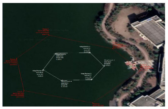
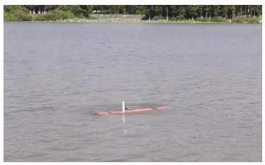
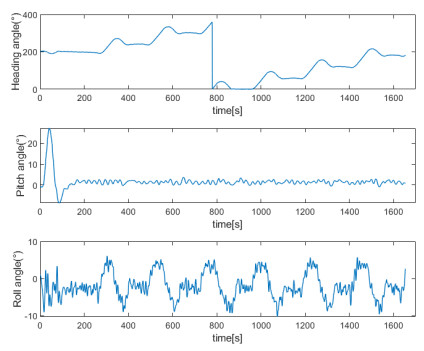
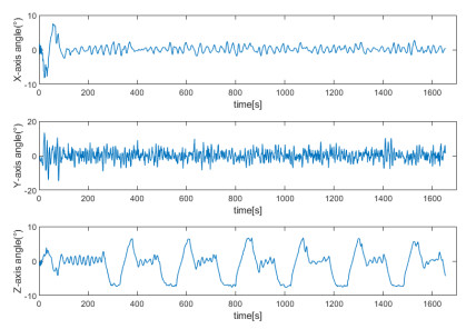
The three-dimensional trajectory tracking of AUV is an important basis for it to complete its task. Due to many uncertain disturbances such as wind, wave and current on the sea, it is easy to cause problems such as slow convergence speed of the controller and saturation of the controller output in the three-dimensional trajectory tracking control of AUV. And the dynamic uncertainty of AUV's own model will have a great negative impact on AUV's trajectory tracking control. In order to solve the problem of slow convergence speed of the above controller, the finite time control method is introduced into the designed position controller. In order to solve the problem of AUV controller output saturation, an auxiliary dynamic system is designed to compensate the system control output saturation. In order to solve the uncertainty of AUV model, a reduced order extended observer is designed in the dynamic controller. It can observe the motion parameters of AUV at any time, and compensate the uncertainty of model uncertainty and external environment disturbance in real time. The control method in this paper is simulated in a three-dimensional model. The experimental results show that the convergence speed, control accuracy, robustness and tracking effect of AUV are higher than those of common trajectory tracker. The algorithm is loaded into the "sea exploration Ⅱ" AUV and verified by experiments in Suzhou lake. The effect of AUV navigation basically meets the task requirements, in which the mean value of pitch angle and heading angle error is less than 8 degrees and the mean value of depth error is less than 0.1M. The trajectory tracker can better meet the trajectory tracking control needs of the AUV.
Citation: Xiaoqiang Dai, Hewei Xu, Hongchao Ma, Jianjun Ding, Qiang Lai. Dual closed loop AUV trajectory tracking control based on finite time and state observer[J]. Mathematical Biosciences and Engineering, 2022, 19(11): 11086-11113. doi: 10.3934/mbe.2022517
The three-dimensional trajectory tracking of AUV is an important basis for it to complete its task. Due to many uncertain disturbances such as wind, wave and current on the sea, it is easy to cause problems such as slow convergence speed of the controller and saturation of the controller output in the three-dimensional trajectory tracking control of AUV. And the dynamic uncertainty of AUV's own model will have a great negative impact on AUV's trajectory tracking control. In order to solve the problem of slow convergence speed of the above controller, the finite time control method is introduced into the designed position controller. In order to solve the problem of AUV controller output saturation, an auxiliary dynamic system is designed to compensate the system control output saturation. In order to solve the uncertainty of AUV model, a reduced order extended observer is designed in the dynamic controller. It can observe the motion parameters of AUV at any time, and compensate the uncertainty of model uncertainty and external environment disturbance in real time. The control method in this paper is simulated in a three-dimensional model. The experimental results show that the convergence speed, control accuracy, robustness and tracking effect of AUV are higher than those of common trajectory tracker. The algorithm is loaded into the "sea exploration Ⅱ" AUV and verified by experiments in Suzhou lake. The effect of AUV navigation basically meets the task requirements, in which the mean value of pitch angle and heading angle error is less than 8 degrees and the mean value of depth error is less than 0.1M. The trajectory tracker can better meet the trajectory tracking control needs of the AUV.

| [1] | W. Caharija, K. Y. Pettersen, J. T. Gravdahl, E. Børhaug, Interal LOS guidance for horizontal path following of underactuated autonomous underwater vehicles in the presence of vertical ocean currents, in 2012 American Control Conference, (2012), 375–382. https://doi.org/10.1109/ACC.2012.6315607 |
| [2] |
P. Encarnacao, A. Pascoal, M. Arcak, Path following for autonomous marine craft, IFAC Proc. Vol., (2000), 117–122. https://doi.org/10.1016/S1474-6670(17)37061-1 doi: 10.1016/S1474-6670(17)37061-1

|
| [3] |
X. Qi, Spatial target path following control based on Nussbaum gain method for underactuated underwater vehicle, Ocean Eng., 104 (2015), 680–685. https://doi.org/10.1016/j.oceaneng.2015.06.014 doi: 10.1016/j.oceaneng.2015.06.014
|
| [4] | H. J. Wang, Z. Y. Chen, H. M. Jia, X. H. Chen, Underactuated AUV 3D path tracking control based filter backstepping method, Acta Autom. Sin., 41 (2015), 631–645. |
| [5] | J. Miao, S. Wang, L. Fan, Y. Li, Spatial curvilinear path following control of underactuated AUV, Acta Armamentarii, 38 (2017), 1786–1796. |
| [6] | J. Gao, W. Yan, N. Zhao, D. Xu, Global path following control for unmanned underwater vehicles, in Proceedings of the 29th Chinese Control Conference, (2010), 3263–3267. |
| [7] |
H. Joe, M. Kim, S. Yu, Second-order sliding-mode controller for autonomous underwater vehicle in the presence of unknown disturbances, Nonlinear Dyn., 78 (2014), 183–196. https://doi.org/10.1007/s11071-014-1431-0 doi: 10.1007/s11071-014-1431-0
|
| [8] | M. Fu, L. Zhou, Y. Xu, Bio-inspired trajectory tracking algorithm based on SFLOS for USV, in 2017 36th Chinese Control Conference, (2017), 26–28. https://doi.org/10.23919/ChiCC.2017.8028143 |
| [9] |
K. D. Do, J. Pan, Z. P. Jiang, Robust and adaptive path following for underactuated autonomous underwater vehicles, Ocean Eng., 104 (2015), 680–685. https://doi.org/10.1016/j.oceaneng.2004.04.006 doi: 10.1016/j.oceaneng.2004.04.006
|
| [10] |
L. Ma, Y. L. Wang, Q. L. Han, Cooperative target tracking of multiple autonomous surface vehicles under switching interaction topologies, IEEE/CAA J. Autom. Sin., (2022). https://doi.org/10.1109/JAS.2022.105509 doi: 10.1109/JAS.2022.105509
|
| [11] |
J. P. Yu, P. Shi, W. J. Dong, C. Lin, Command filteringbased fuzzy control for nonlinear systems with saturation input, IEEE Trans. Cybern, 9 (2017), 2472–2479. https://doi.org/10.1109/TCYB.2016.2633367 doi: 10.1109/TCYB.2016.2633367
|
| [12] |
J. Wang, C. Wang, Y. Wei, C. Zhang, Command filter based adaptive neural trajectory tracking control of an underactuated underwater vehicle in three-dimesional space, Ocean Eng., 180 (2019), 175–186. https://doi.org/10.1016/j.oceaneng.2019.03.061 doi: 10.1016/j.oceaneng.2019.03.061
|
| [13] |
X. Jin, Fault tolerant finite-time leader-follower formation control for autonomous surface vessels with LOS range and angle constraints, Automatica, 68 (2016), 228–236. https://doi.org/10.1016/j.automatica.2016.01.064 doi: 10.1016/j.automatica.2016.01.064
|
| [14] | D. A. Nguyen, D. D. Thanh, N. T. Tien, P. V. Anh, Fuzzy Controller Design for Autonomous Underwater Vehicles Path Tracking, in Proceedings of 2019 International Conference on System Science and Engineering, ICSSE, (2019), 592–598. https://doi.org/10.1109/ICSSE.2019.8823333 |
| [15] | M. H. A. Majid, M. R. Arshad, A fuzzy self-adaptive PID tracking control of autonomous surface vehicle, in 2015 IEEE International Conference on Control System, Computing and Engineering, (2015), 458–463. https://doi.org/10.1109/ICCSCE.2015.7482229 |
| [16] |
A.Bagheri, T.Karimi, N.Amanifard, Tracking performance control of a cable communicated underwater vehicle using adaptive neural network controllers, Appl. Soft Comput., 10 (2010), 908–918. https://doi.org/10.1016/j.asoc.2009.10.008 doi: 10.1016/j.asoc.2009.10.008
|
| [17] |
L. Zhang, X. Qi, Y. Pang, Adaptive output feedback control based on DRFNN for UUV, Ocean Eng., 36 (2009), 716–722. https://doi.org/10.1016/j.oceaneng.2009.03.011 doi: 10.1016/j.oceaneng.2009.03.011
|
| [18] |
T. Elmokadem, M. Zribi, K. Youcef-Toumi, Trajectory tracking sliding mode control of underactuated AUVs, Nonlinear Dyn., 84 (2016), 1079–1091. https://doi.org/10.1007/s11071-015-2551-x doi: 10.1007/s11071-015-2551-x
|
| [19] |
E. Zakeri, S. Farahat, S. A. Moezi, A. Zare, Robust sliding mode control of a miniunmanned enderwater vehicle equipped with a new arrangement of water jetpropulsions: Simulation and experimental study, Appl. Ocean Res., 59 (2016), 521–542. https://doi.org/10.1016/j.apor.2016.07.006 doi: 10.1016/j.apor.2016.07.006
|
| [20] |
T. Elmokadem, M. Zribi, K. Youcef-Toumi, Terminal sliding mode control for the trajectory tracking of underactuated Autonomous Underwater Vehicles, Ocean Eng., 129 (2017), 613–625. https://doi.org/10.1016/j.oceaneng.2016.10.032 doi: 10.1016/j.oceaneng.2016.10.032
|
| [21] |
Y. Wang, L. Gu, M. Gao, K. Zhu, Multivariable output feedback adaptive terminal sliding mode control for underwater vehicles, Asian J. Control, 18(1) (2016), 247–265. https://doi.org/10.1002/asjc.1013 doi: 10.1002/asjc.1013
|
| [22] |
N. Ali, I. Tawiah, W. Zhang, Finite-time extended state observer based nonsinglar fast terminal sliding mode control of autonomous underwater vehicles, Ocean Eng., 281 (2020), 108179. https://doi.org/10.1016/j.oceaneng.2020.108179 doi: 10.1016/j.oceaneng.2020.108179
|

Figures(15) / Tables(10)

Xiaoqiang Dai, Hewei Xu, Hongchao Ma, Jianjun Ding, Qiang Lai. Dual closed loop AUV trajectory tracking control based on finite time and state observer[J]. Mathematical Biosciences and Engineering, 2022, 19(11): 11086-11113. doi: 10.3934/mbe.2022517


 DownLoad: