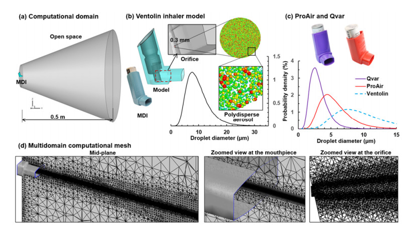
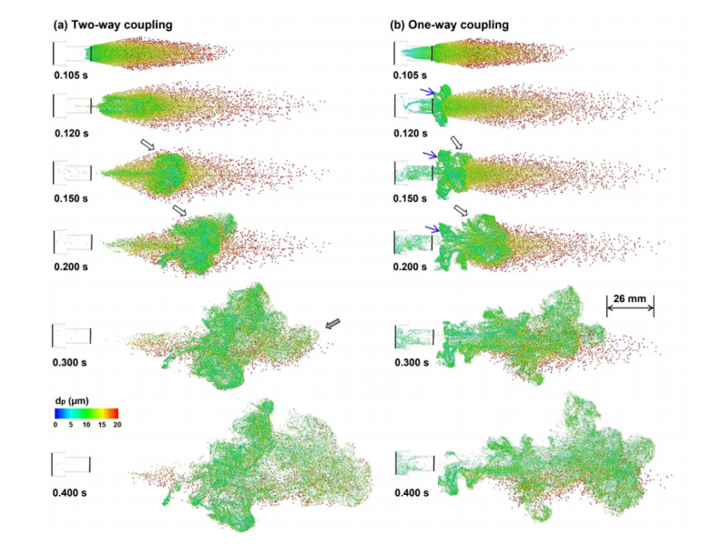
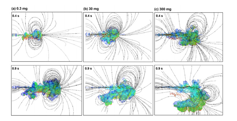
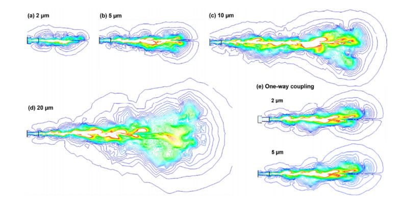
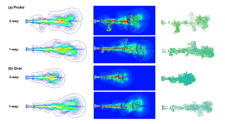
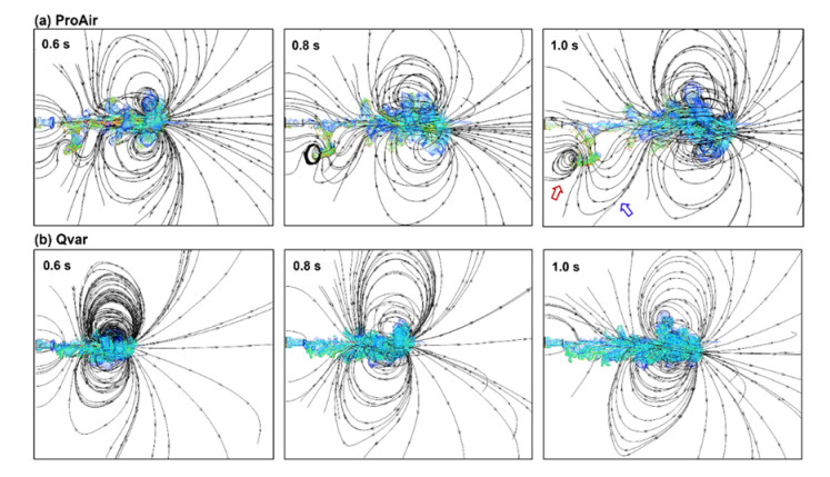
Previous numerical studies of pulmonary drug delivery using metered-dose inhalers (MDIs) often neglected the momentum transfer from droplets to fluid. However, Kolmogorov length scales in MDI flows can be comparable to the droplet sizes in the orifice vicinity, and their interactions can modify the spray behaviors. This study aimed to evaluate the two-way coupling effects on spray plume evolutions compared to one-way coupling. The influences from the mass loading, droplet size, and inhaler type were also examined. Large-eddy simulation and Lagrangian approach were used to simulate the flow and droplet motions. Two-way coupled predictions appeared to provide significantly improved predictions of the aerosol behaviors close to the Ventolin orifice than one-way coupling. Increasing the applied MDI dose mass altered both the fluid and aerosol dynamics, notably bending the spray plume downward when applying a dose ten times larger. The droplet size played a key role in spray dynamics, with the plume being suppressed for 2-µm aerosols and enhanced for 20-µm aerosols. The Kolmogorov length scale ratio dp/η correlated well with the observed difference in spray plumes, with suppressed plumes when dp/η < 0.1 and enhanced plumes when dp/η > 0.1. For the three inhalers considered (Ventolin, ProAir, and Qvar), significant differences were predicted using two-way and one-way coupling despite the level and manifestation of these differences varied. Two-way coupling effects were significant for MDI sprays and should be considered in future numerical studies.
Citation: Jinxiang Xi, Mohamed Talaat, Xiuhua April Si. Two-way coupling and Kolmogorov scales on inhaler spray plume evolutions from Ventolin, ProAir, and Qvar[J]. Mathematical Biosciences and Engineering, 2022, 19(11): 10915-10940. doi: 10.3934/mbe.2022510
Previous numerical studies of pulmonary drug delivery using metered-dose inhalers (MDIs) often neglected the momentum transfer from droplets to fluid. However, Kolmogorov length scales in MDI flows can be comparable to the droplet sizes in the orifice vicinity, and their interactions can modify the spray behaviors. This study aimed to evaluate the two-way coupling effects on spray plume evolutions compared to one-way coupling. The influences from the mass loading, droplet size, and inhaler type were also examined. Large-eddy simulation and Lagrangian approach were used to simulate the flow and droplet motions. Two-way coupled predictions appeared to provide significantly improved predictions of the aerosol behaviors close to the Ventolin orifice than one-way coupling. Increasing the applied MDI dose mass altered both the fluid and aerosol dynamics, notably bending the spray plume downward when applying a dose ten times larger. The droplet size played a key role in spray dynamics, with the plume being suppressed for 2-µm aerosols and enhanced for 20-µm aerosols. The Kolmogorov length scale ratio dp/η correlated well with the observed difference in spray plumes, with suppressed plumes when dp/η < 0.1 and enhanced plumes when dp/η > 0.1. For the three inhalers considered (Ventolin, ProAir, and Qvar), significant differences were predicted using two-way and one-way coupling despite the level and manifestation of these differences varied. Two-way coupling effects were significant for MDI sprays and should be considered in future numerical studies.

| [1] |
X. Si, M. Talaat, J. Xi, SARS COV-2 virus-laden droplets coughed from deep lungs: Numerical quantification in a single-path whole respiratory tract geometry, Phys. Fluids, 33 (2021), 23306. https://doi.org/10.1063/5.0040914 doi: 10.1063/5.0040914

|
| [2] |
P. W. Longest, S. Vinchurkar, T. B. Martonen, Transport and deposition of respiratory aerosols in models of childhood asthma, J. Aerosol Sci., 37 (2006), 1234–1257. https://doi.org/10.1016/j.jaerosci.2006.01.011 doi: 10.1016/j.jaerosci.2006.01.011
|
| [3] |
C. Kleinstreuer, H. Shi, Z. Zhang, Computational analyses of a pressurized metered dose inhaler and a new drug-aerosol targeting methodology, J. Aerosol Med., 20 (2007), 294–309. https://doi.org/10.1089/jam.2006.0617 doi: 10.1089/jam.2006.0617
|
| [4] |
H. Smyth, G. Brace, T. Barbour, J. Gallion, J. Grove, A. J. Hickey, Spray pattern analysis for metered dose inhalers: Effect of actuator design, Pharm. Res., 23 (2006), 1591–1596. https://doi.org/10.1007/s11095-006-0280-z doi: 10.1007/s11095-006-0280-z
|
| [5] |
H. K. Versteeg, G. K. Hargrave, M. Kirby, Internal flow and near-orifice spray visualisations of a model pharmaceutical pressurised metered dose inhaler, J. Phys. Conf. Ser., 45 (2006), 207–213. https://doi.org/10.1088/1742-6596/45/1/028 doi: 10.1088/1742-6596/45/1/028
|
| [6] |
H. Smyth, A. J. Hickey, G. Brace, T. Barbour, J. Gallion, J. Grove, Spray pattern analysis for metered dose inhalers Ⅰ: Orifice size, particle size, and droplet motion correlations, Drug Dev. Ind. Pharm., 32 (2006), 1033–1041. https://doi.org/10.1080/03639040600637598 doi: 10.1080/03639040600637598
|
| [7] |
L. B. Torobin, W. H. Gauvin, Fundamental aspects of solids-gas flow: Part Ⅵ: Multiparticle behavior in turbulent fluids, Can. J. Chem. Eng., 39 (1961), 113–120. https://doi.org/10.1002/cjce.5450390304 doi: 10.1002/cjce.5450390304
|
| [8] |
G. Gai, A. Hadjadj, S. Kudriakov, O. Thomine, Particles-induced turbulence: A critical review of physical concepts, numerical modelings and experimental investigations, Theor. Appl. Mech. Lett., 10 (2020), 241–248. https://doi.org/10.1016/j.taml.2020.01.026 doi: 10.1016/j.taml.2020.01.026
|
| [9] |
M. Pan, C. Liu, Q. Li, S. Tang, L. Shen, Y. Dong, Impact of spray droplets on momentum and heat transport in a turbulent marine atmospheric boundary layer, Theor. Appl. Mech. Lett., 9 (2019), 71–78. https://doi.org/10.1016/j.taml.2019.02.002 doi: 10.1016/j.taml.2019.02.002
|
| [10] |
R. A. Gore, C. T. Crowe, Effect of particle size on modulating turbulent intensity, Int. J. Multiph. Flow, 15 (1989), 279–285. https://doi.org/10.1016/0301-9322(89)90076-1 doi: 10.1016/0301-9322(89)90076-1
|
| [11] | C. T. Crowe, J. D. Schwarzkopf, M. Sommerfeld, Y. Tsuji, Multiphase Flows with Droplets and Particles, CRC Press, 2011. https://doi.org/10.1201/b11103 |
| [12] |
S. Elghobashi, G. Truesdell, On the two-way interaction between homogeneous turbulence and dispersed solid particles. Ⅰ: Turbulence modification, Phys. Fluids, 5 (1993), 1790–1801. https://doi.org/10.1063/1.858854 doi: 10.1063/1.858854
|
| [13] |
M. Di Giacinto, F. Sabetta, R. Piva, Two-way coupling effects in dilute gas-particle flows, J. Fluids Eng., 104 (1982), 304–311. https://doi.org/10.1115/1.3241836 doi: 10.1115/1.3241836
|
| [14] |
R. Monchaux, A. Dejoan, Settling velocity and preferential concentration of heavy particles under two-way coupling effects in homogeneous turbulence, Phys. Rev. Fluids, 2 (2017), 104302. https://doi.org/10.1103/PhysRevFluids.2.104302 doi: 10.1103/PhysRevFluids.2.104302
|
| [15] |
S. Elghobashi, On predicting particle-laden turbulent flows, Appl. Sci. Res., 52 (1994), 309–329. https://doi.org/10.1007/BF00936835 doi: 10.1007/BF00936835
|
| [16] |
B. J. Gabrio, S. W. Stein, D. J. Velasquez, A new method to evaluate plume characteristics of hydrofluoroalkane and chlorofluorocarbon metered dose inhalers, Int. J. Pharm., 186 (1999), 3–12. https://doi.org/10.1016/s0378-5173(99)00133-7 doi: 10.1016/s0378-5173(99)00133-7
|
| [17] |
X. Liu, W. H. Doub, C. Guo, Evaluation of metered dose inhaler spray velocities using phase Doppler anemometry (PDA), Int. J. Pharm., 423 (2012), 235–239. https://doi.org/10.1016/j.ijpharm.2011.12.006 doi: 10.1016/j.ijpharm.2011.12.006
|
| [18] |
M. Talaat, X. Si, J. Xi, Effect of MDI actuation timing on inhalation dosimetry in a human respiratory tract model, Pharmaceuticals, 15 (2022), 61. https://doi.org/10.3390/ph15010061 doi: 10.3390/ph15010061
|
| [19] |
A. Alatrash, E. Matida, Characterization of medication velocity and size distribution from pressurized metered-dose inhalers by phase Doppler anemometry, J. Aerosol Med. Pulm. Drug Deliv., 29 (2016), 501–513. https://doi.org/10.1089/jamp.2015.1264 doi: 10.1089/jamp.2015.1264
|
| [20] |
S. Suissa, P. Ernst, J. F. Boivin, R. I. Horwitz, B. Habbick, D. Cockroft, et al., A cohort analysis of excess mortality in asthma and the use of inhaled beta-agonists, Am. J. Respir. Crit. Care Med., 149 (1994), 604–610. https://doi.org/10.1164/ajrccm.149.3.8118625 doi: 10.1164/ajrccm.149.3.8118625
|
| [21] |
S. Newman, A. Salmon, R. Nave, A. Drollmann, High lung deposition of 99mTc-labeled ciclesonide administered via HFA-MDI to patients with asthma, Respir. Med., 100 (2006), 375–384. https://doi.org/10.1016/j.rmed.2005.09.027 doi: 10.1016/j.rmed.2005.09.027
|
| [22] |
R. H. Hatley, D. von Hollen, D. Sandell, L. Slator, In vitro characterization of the OptiChamber Diamond valved holding chamber, J. Aerosol Med. Pulm. Drug Deliv., 27 Suppl 1 (2014), S24–36. https://doi.org/10.1089/jamp.2013.1067 doi: 10.1089/jamp.2013.1067
|
| [23] |
F. M. Shemirani, S. Hoe, D. Lewis, T. Church, R. Vehring, W. H. Finlay, In vitro investigation of the effect of ambient humidity on regional delivered dose with solution and suspension MDIs, J. Aerosol Med. Pulm. Drug Deliv., 26 (2013), 215–222. https://doi.org/10.1089/jamp.2012.0991 doi: 10.1089/jamp.2012.0991
|
| [24] |
R. Marijani, M. S. Shaik, A. Chatterjee, M. Singh, Evaluation of metered dose inhaler (MDI) formulations of ciclosporin, J. Pharm. Pharmacol., 59 (2007), 15–21. https://doi.org/10.1211/jpp.59.1.0003 doi: 10.1211/jpp.59.1.0003
|
| [25] |
F. Nicoud, F. Ducros, Subgrid-scale stress modelling based on the square of the velocity gradient tensor, Flow Turbul. Combust., 62 (1999), 183–200. https://doi.org/10.1023/a:1009995426001 doi: 10.1023/a:1009995426001
|
| [26] |
P. W. Longest, J. Xi, Effectiveness of direct Lagrangian tracking models for simulating nanoparticle deposition in the upper airways, Aerosol Sci. Tech., 41 (2007), 380–397. https://doi.org/10.1080/02786820701203223 doi: 10.1080/02786820701203223
|
| [27] |
J. Kim, J. Xi, X. Si, A. Berlinski, W. C. Su, Hood nebulization: Effects of head direction and breathing mode on particle inhalability and deposition in a 7-month-old infant model, J. Aerosol Med. Pulm. Drug Deliv., 27 (2014), 209–218. https://doi.org/10.1089/jamp.2013.1051 doi: 10.1089/jamp.2013.1051
|
| [28] |
C. A. Ruzycki, E. Javaheri, W. H. Finlay, The use of computational fluid dynamics in inhaler design, Expert Opin. Drug Deliv., 10 (2013), 307–323. https://doi.org/10.1517/17425247.2013.753053 doi: 10.1517/17425247.2013.753053
|
| [29] |
P. W. Longest, G. Tian, R. L. Walenga, M. Hindle, Comparing MDI and DPI aerosol deposition using in vitro experiments and a new stochastic individual path (SIP) model of the conducting airways, Pharm. Res., 29 (2012), 1670–1688. https://doi.org/10.1007/s11095-012-0691-y doi: 10.1007/s11095-012-0691-y
|
| [30] |
M. Talaat, X. Si, J. Xi, Lower inspiratory breathing depth enhances pulmonary delivery efficiency of ProAir sprays, Pharmaceuticals, 15 (2022), 706. https://doi.org/10.3390/ph15060706 doi: 10.3390/ph15060706
|
| [31] |
L. Schneiders, M. Meinke, W. Schröder, Direct particle-fluid simulation of Kolmogorov-length-scale size particles in decaying isotropic turbulence, J. Fluid Mech., 819 (2017), 188–227. https://doi.org/10.1017/jfm.2017.171 doi: 10.1017/jfm.2017.171
|
| [32] | M. T. Landahl, E. Mollo-Christensen, Turbulence and Random Processes in Fluid Mechanics, 2nd edition, Cambridge University Press, Cambridge, 1992. https://doi.org/10.1017/9781139174008 |
| [33] |
R. F. Huang, J. Lan, Characteristic modes and evolution processes of shear-layer vortices in an elevated transverse jet, Phys. Fluids, 17 (2005), 34103. https://doi.org/10.1063/1.1852575 doi: 10.1063/1.1852575
|
| [34] |
T. T. Lim, T. H. New, S. C. Luo, On the development of large-scale structures of a jet normal to a cross flow, Phys. Fluids, 13 (2001), 770–775. https://doi.org/10.1063/1.1347960 doi: 10.1063/1.1347960
|
| [35] |
T. H. New, J. Long, Dynamics of laminar circular jet impingement upon convex cylinders, Phys. Fluids, 27 (2015), 24109. https://doi.org/10.1063/1.4913498 doi: 10.1063/1.4913498
|
| [36] |
X. L. Tong, L. P. Wang, Two-way coupled particle-laden mixing layer. Part 1: Linear instability, Int. J. Multiph. Flow, 25 (1999), 575–598. https://doi.org/10.1016/S0301-9322(98)00059-7 doi: 10.1016/S0301-9322(98)00059-7
|
| [37] |
H. Nasr, G. Ahmadi, The effect of two-way coupling and inter-particle collisions on turbulence modulation in a vertical channel flow, Int. J. Heat Fluid Flow, 28 (2007), 1507–1517. https://doi.org/10.1016/j.ijheatfluidflow.2007.03.007 doi: 10.1016/j.ijheatfluidflow.2007.03.007
|
| [38] |
R. H. A. IJzermans, R. Hagmeijer, Accumulation of heavy particles in N-vortex flow on a disk, Phys. Fluids, 18 (2006), 063601. https://doi.org/10.1063/1.2212987 doi: 10.1063/1.2212987
|
| [39] |
G. Hetsroni, Particles-turbulence interaction, Int. J. Multiph. Flow, 15 (1989), 735–746. https://doi.org/10.1016/0301-9322(89)90037-2 doi: 10.1016/0301-9322(89)90037-2
|
| [40] |
Z. Yuan, E. E. Michaelides, Turbulence modulation in particulate flows—A theoretical approach, Int. J. Multiph. Flow, 18 (1992), 779–785. https://doi.org/10.1016/0301-9322(92)90045-I doi: 10.1016/0301-9322(92)90045-I
|
| [41] |
C. T. Crowe, On models for turbulence modulation in fluid-particle flows, Int. J. Multiph. Flow, 26 (2000), 719–727. https://doi.org/10.1016/S0301-9322(99)00050-6 doi: 10.1016/S0301-9322(99)00050-6
|
| [42] |
C. He, G. Ahmadi, Particle deposition with thermophoresis in laminar and turbulent duct flows, Aerosol Sci. Tech., 29 (1998), 525–546. https://doi.org/10.1080/02786829808965588 doi: 10.1080/02786829808965588
|
| [43] |
Z. Q. Yin, X. F. Li, F. B. Bao, C. X. Tu, X. Y. Gao, Thermophoresis and Brownian motion effects on nanoparticle deposition inside a 90° square bend tube, Aerosol Air Qual. Res., 18 (2018), 1746–1755. https://doi.org/10.4209/aaqr.2018.02.0047 doi: 10.4209/aaqr.2018.02.0047
|
| [44] |
J. Xi, J. Kim, X. A. Si, Y. Zhou, Hygroscopic aerosol deposition in the human upper respiratory tract under various thermo-humidity conditions, J. Environ. Sci. Heal. A, 48 (2013), 1790–1805. https://doi.org/10.1080/10934529.2013.823333 doi: 10.1080/10934529.2013.823333
|
| [45] |
J. W. Kim, J. Xi, X. A. Si, Dynamic growth and deposition of hygroscopic aerosols in the nasal airway of a 5-year-old child, Int. J. Numer. Methods Biomed. Eng., 29 (2013), 17–39. https://doi.org/10.1002/cnm.2490 doi: 10.1002/cnm.2490
|
| [46] |
P. W. Longest, J. Xi, Condensational growth may contribute to the enhanced deposition of cigarette smoke particles in the upper respiratory tract, Aerosol Sci. Tech., 42 (2008), 579–602. https://doi.org/10.1080/02786820802232964 doi: 10.1080/02786820802232964
|
| [47] |
G. Tian, P. W. Longest, G. Su, M. Hindle, Characterization of respiratory drug delivery with enhanced condensational growth using an individual path model of the entire tracheobronchial airways, Ann. Biomed. Eng., 39 (2011), 1136–1153. https://doi.org/10.1007/s10439-010-0223-z doi: 10.1007/s10439-010-0223-z
|
| [48] |
J. Xi, X. Si, P. W. Longest, Electrostatic charge effects on pharmaceutical aerosol deposition in human nasal-laryngeal airways, Pharmaceutics, 6 (2013), 26–35. https://doi.org/10.3390/pharmaceutics6010026 doi: 10.3390/pharmaceutics6010026
|
| [49] |
J. Xi, J. Eddie Yuan, M. Alshaiba, D. Cheng, Z. Firlit, A. Johnson, et al., Design and testing of electric-guided delivery of charged particles to the olfactory region: Experimental and numerical studies, Curr. Drug Deliv., 13 (2016), 265–274. https://doi.org/10.2174/1567201812666150909093050 doi: 10.2174/1567201812666150909093050
|
| [50] |
J. Xi, J. E. Yuan, X. A. Si, J. Hasbany, Numerical optimization of targeted delivery of charged nanoparticles to the ostiomeatal complex for treatment of rhinosinusitis, Int. J. Nanomedicine, 10 (2015), 4847–4861. https://doi.org/10.2147/IJN.S87382 doi: 10.2147/IJN.S87382
|
| [51] |
M. Azhdarzadeh, J. S. Olfert, R. Vehring, W. H. Finlay, Effect of electrostatic charge on deposition of uniformly charged monodisperse particles in the nasal extrathoracic airways of an infant, J. Aerosol Med. Pulm. Drug Deliv., 28 (2015), 30–34. https://doi.org/10.1089/jamp.2013.1118 doi: 10.1089/jamp.2013.1118
|
| [52] |
P. G. Koullapis, S. C. Kassinos, M. P. Bivolarova, A. K. Melikov, Particle deposition in a realistic geometry of the human conducting airways: Effects of inlet velocity profile, inhalation flowrate and electrostatic charge, J. Biomech., 49 (2016), 2201–2212. https://doi.org/10.1016/j.jbiomech.2015.11.029 doi: 10.1016/j.jbiomech.2015.11.029
|
| [53] |
J. Xi, Z. Wang, K. Talaat, C. Glide-Hurst, H. Dong, Numerical study of dynamic glottis and tidal breathing on respiratory sounds in a human upper airway model, Sleep Breath., 22 (2018), 463–479. https://doi.org/10.1007/s11325-017-1588-0 doi: 10.1007/s11325-017-1588-0
|
| [54] |
J. Zhao, Y. Feng, C. A. Fromen, Glottis motion effects on the particle transport and deposition in a subject-specific mouth-to-trachea model: A CFPD study, Comput. Biol. Med., 116 (2020), 103532. https://doi.org/10.1016/j.compbiomed.2019.103532 doi: 10.1016/j.compbiomed.2019.103532
|
| [55] |
M. Triep, C. Brücker, Three-dimensional nature of the glottal jet, J. Acoust. Soc. Am., 127 (2010), 1537–1547. https://doi.org/10.1121/1.3299202 doi: 10.1121/1.3299202
|
| [56] |
L. Bailly, T. Cochereau, L. Orgéas, N. Henrich Bernardoni, S. Rolland du Roscoat, A. Mcleer-Florin, et al., 3D multiscale imaging of human vocal folds using synchrotron X-ray microtomography in phase retrieval mode, Sci. Rep., 8 (2018), 1–20. https://doi.org/10.1038/s41598-018-31849-w doi: 10.1038/s41598-018-31849-w
|
Figures(14) / Tables(2)

Jinxiang Xi, Mohamed Talaat, Xiuhua April Si. Two-way coupling and Kolmogorov scales on inhaler spray plume evolutions from Ventolin, ProAir, and Qvar[J]. Mathematical Biosciences and Engineering, 2022, 19(11): 10915-10940. doi: 10.3934/mbe.2022510


 DownLoad: