Isolation in the control of epidemic

Yong Zhou; Minrui Guo; Yong Zhou; Minrui Guo

doi:10.3934/mbe.2022507

Mathematical Biosciences and Engineering

2022, Volume 19, Issue 11: 10846-10863. doi: 10.3934/mbe.2022507

Previous Article Next Article

Research article

Isolation in the control of epidemic

Yong Zhou ^{1
,
,},
Minrui Guo ²

1.
College of Science, Wuhan University of Science and Technology, Wuhan 430065, China
2.
College of Energy Engineering, Huanghuai University, Zhumadian 463000, China

Received: 25 May 2022 Revised: 26 July 2022 Accepted: 27 July 2022 Published: 29 July 2022

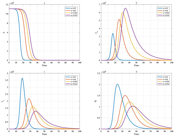
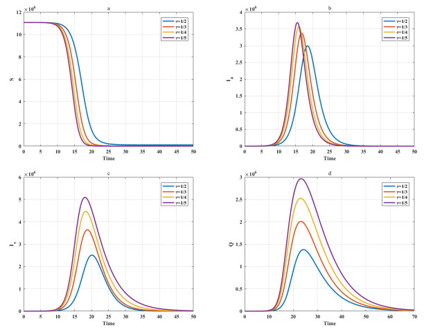
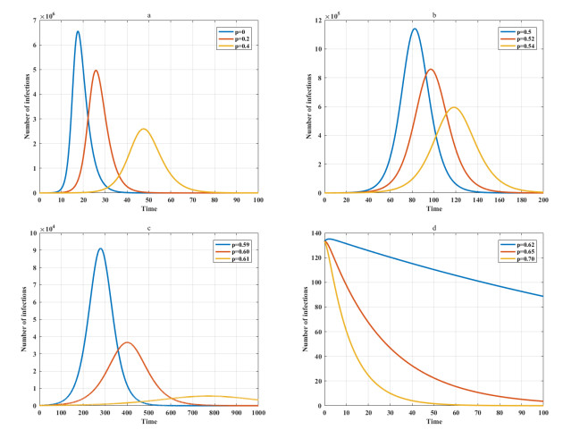
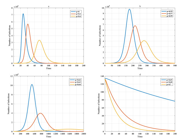
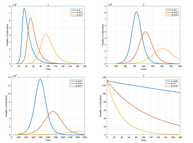
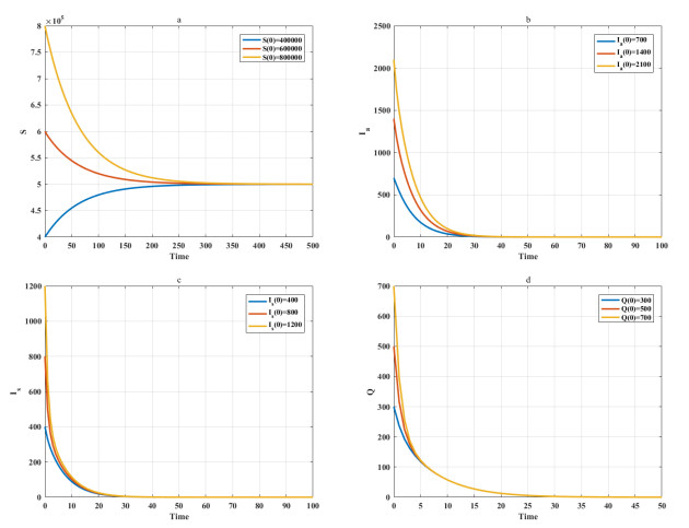
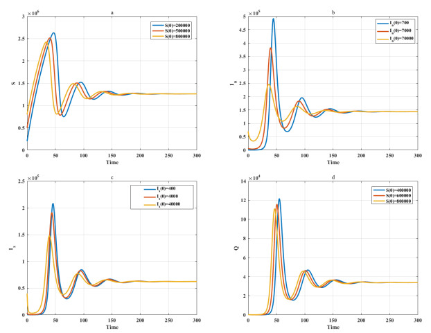
Among many epidemic prevention measures, isolation is an important method to control the spread of infectious disease. Scholars rarely study the impact of isolation on disease dissemination from a quantitative perspective. In this paper, we introduce an isolation ratio and establish the corresponding model. The basic reproductive number and its biological explanation are given. The stability conditions of the disease-free and endemic equilibria are obtained by analyzing its distribution of characteristic values. It is shown that the isolation ratio has an important influence on the basic reproductive number and the stability conditions. Taking the COVID-19 in Wuhan as an example, isolating more than 68% of the population can control the spread of the epidemic. This method can provide precise epidemic prevention strategies for government departments. Numerical simulations verify the effectiveness of the results.
- epidemic,
- isolation ratio,
- basic reproductive number,
- stability of equilibrium
Citation: Yong Zhou, Minrui Guo. Isolation in the control of epidemic[J]. Mathematical Biosciences and Engineering, 2022, 19(11): 10846-10863. doi: 10.3934/mbe.2022507

Related Papers:

Abstract

Among many epidemic prevention measures, isolation is an important method to control the spread of infectious disease. Scholars rarely study the impact of isolation on disease dissemination from a quantitative perspective. In this paper, we introduce an isolation ratio and establish the corresponding model. The basic reproductive number and its biological explanation are given. The stability conditions of the disease-free and endemic equilibria are obtained by analyzing its distribution of characteristic values. It is shown that the isolation ratio has an important influence on the basic reproductive number and the stability conditions. Taking the COVID-19 in Wuhan as an example, isolating more than 68% of the population can control the spread of the epidemic. This method can provide precise epidemic prevention strategies for government departments. Numerical simulations verify the effectiveness of the results.

References

[1]	H. Wang, Z. Wang, Y. Dong, R. Chang, C. Xu, X. Yu, et al., Phase-adjusted estimation of the number of coronavirus disease 2019 cases in wuhan, china, Cell Discov., 6 (2020), 1–8. https://doi.org/10.1038/s41421-020-0148-0 doi: 10.1038/s41421-020-0148-0
[2]	D. Wang, M. Zhou, X. Nie, W. Qiu, M. Yang, X. Wang, et al., Epidemiological characteristics and transmission model of corona virus disease 2019 in china, J. Infect., 80 (2020), e25–e27. https://doi.org/10.1016/j.jinf.2020.03.008 doi: 10.1016/j.jinf.2020.03.008
[3]	F. S. Dawood, P. Ricks, G. J. Njie, M. Daugherty, W. Davis, J. A. Fuller, et al., Observations of the global epidemiology of covid-19 from the prepandemic period using web-based surveillance: A cross-sectional analysis, Lancet Infect. Dis., 20 (2020), 1255–1262. https://doi.org/10.1016/S1473-3099(20)30581-8 doi: 10.1016/S1473-3099(20)30581-8
[4]	C. Jiang, X. Li, C. Ge, Y. Ding, T. Zhang, S. Cao, et al., Molecular detection of sars-cov-2 being challenged by virus variation and asymptomatic infection, J. Pharm. Anal., 11 (2021), 257–264. https://doi.org/10.1016/j.jpha.2021.03.006 doi: 10.1016/j.jpha.2021.03.006
[5]	F. A. Engelbrecht, R. J. Scholes, Test for covid-19 seasonality and the risk of second waves, One Health, 12 (2021), 100202.
[6]	M. Yao, H. Wang, A potential treatment for covid-19 based on modal characteristics and dynamic responses analysis of 2019-ncov, Nonlinear Dyn., 106 (2021), 1425–1432. https://doi.org/10.1007/s11071-020-06019-1 doi: 10.1007/s11071-020-06019-1
[7]	P. Das, R. K. Upadhyay, A. K. Misra, F. A. Rihan, P. Das, D. Ghosh, Mathematical model of covid-19 with comorbidity and controlling using non-pharmaceutical interventions and vaccination, Nonlinear Dyn., 106 (2021), 1213–1227. https://doi.org/10.1007/s11071-021-06517-w doi: 10.1007/s11071-021-06517-w
[8]	K. Shah, Z. A. Khan, A. Ali, R. Amin, H. Khan, A. Khan, Haar wavelet collocation approach for the solution of fractional order covid-19 model using caputo derivative, Alex. Eng. J., 59 (2020), 3221–3231. https://doi.org/10.1016/j.aej.2020.08.028 doi: 10.1016/j.aej.2020.08.028
[9]	C. Han, Y. Liu, J. Tang, Y. Zhu, C. Jaeger, S. Yang, Lessons from the mainland of China's epidemic experience in the first phase about the growth rules of infected and recovered cases of covid-19 worldwide, Int. J. Disaster Risk Sci., 11 (2020), 497–507. https://doi.org/10.1007/s13753-020-00294-7 doi: 10.1007/s13753-020-00294-7
[10]	J. T. Machado, J. Ma, Nonlinear dynamics of covid-19 pandemic: modeling, control, and future perspectives, Nonlinear Dyn., 101 (2020), 1525–1526. https://doi.org/10.1007/s11071-020-05919-6 doi: 10.1007/s11071-020-05919-6
[11]	S. He, Y. Peng, K. Sun, Seir modeling of the covid-19 and its dynamics, Nonlinear Dyn., 101 (2020), 1667–1680. https://doi.org/10.1007/s11071-020-05743-y doi: 10.1007/s11071-020-05743-y
[12]	G. Stewart, K. van Heusden, G. A. Dumont, How control theory can help us control covid-19, IEEE Spectrum, 57 (2020), 22–29. https://doi.org/10.1109/MSPEC.2020.9099929 doi: 10.1109/MSPEC.2020.9099929
[13]	D. Fanelli, F. Piazza, Analysis and forecast of covid-19 spreading in china, italy and france, Chaos Solitons Fract., 134 (2020), 109761.
[14]	R. Li, S. Pei, B. Chen, Y. Song, T. Zhang, W. Yang et al., Substantial undocumented infection facilitates the rapid dissemination of novel coronavirus (sars-cov-2), Science, 368 (2020), 489–493.
[15]	W. O. Kermack, A. G. McKendrick, Contributions to the mathematical theory of epidemics. ii.—the problem of endemicity, Bull. Math. Biol., 138 (1932), 55–83.
[16]	C. Zheng, Complex network propagation effect based on sirs model and research on the necessity of smart city credit system construction, Alex. Eng. J., 61 (2022), 403–418. https://doi.org/10.1016/j.aej.2021.06.004 doi: 10.1016/j.aej.2021.06.004
[17]	Z. Zhao, L. Pang, Y. Chen, Nonsynchronous bifurcation of sirs epidemic model with birth pulse and pulse vaccination, Nonlinear Dyn., 79 (2015), 2371–2383. https://doi.org/10.1007/s11071-014-1818-y doi: 10.1007/s11071-014-1818-y
[18]	D. Saikia, K. Bora, M. P. Bora, Covid-19 outbreak in india: An seir model-based analysis, Nonlinear Dyn., 104 (2021), 4727–4751.
[19]	C. Xu, Y. Yu, Y. Chen, Z. Lu, Forecast analysis of the epidemics trend of covid-19 in the usa by a generalized fractional-order seir model, Nonlinear Dyn., 101 (2020), 1621–1634. https://doi.org/10.1007/s11071-020-05946-3 doi: 10.1007/s11071-020-05946-3
[20]	R. K. Upadhyay, A. K. Pal, S. Kumari, P. Roy, Dynamics of an seir epidemic model with nonlinear incidence and treatment rates, Nonlinear Dyn., 96 (2019), 2351–2368. https://doi.org/10.1007/s11071-019-04926-6 doi: 10.1007/s11071-019-04926-6
[21]	P. Yarsky, Using a genetic algorithm to fit parameters of a covid-19 seir model for us states, Math. Comput. Simulat., 185 (2021), 687–695. https://doi.org/10.1016/j.matcom.2021.01.022 doi: 10.1016/j.matcom.2021.01.022
[22]	N. ben Khedher, L. Kolsi, H. Alsaif, A multi-stage seir model to predict the potential of a new covid-19 wave in ksa after lifting all travel restrictions, Alex. Eng. J., 60 (2021), 3965–3974. https://doi.org/10.1016/j.aej.2021.02.058 doi: 10.1016/j.aej.2021.02.058
[23]	N. Piovella, Analytical solution of seir model describing the free spread of the covid-19 pandemic, Chaos Solitons Fract., 140 (2020), 110243.
[24]	S. J. Weinstein, M. S. Holland, K. E. Rogers, N. S. Barlow, Analytic solution of the seir epidemic model via asymptotic approximant, Physica D., 411 (2020), 132633–132633. https://doi.org/10.1016/j.physd.2020.132633 doi: 10.1016/j.physd.2020.132633
[25]	T. Britton, D. Ouédraogo, Seirs epidemics with disease fatalities in growing populations., Math. Biosci., 296 (2018), 45–59. https://doi.org/10.1016/j.mbs.2017.11.006 doi: 10.1016/j.mbs.2017.11.006
[26]	G. Lu, Z. Lu, Global asymptotic stability for the seirs models with varying total population size., Math. Biosci., 296 (2018), 17–25. https://doi.org/10.1016/j.mbs.2017.11.010 doi: 10.1016/j.mbs.2017.11.010
[27]	O. M. Otunuga, Estimation of epidemiological parameters for covid-19 cases using a stochastic seirs epidemic model with vital dynamics, Result. Phys., 28 (2021), 104664.
[28]	M. A. Abdelaziz, A. I. Ismail, F. A. Abdullah, M. H. Mohd, Codimension one and two bifurcations of a discrete-time fractional-order seir measles epidemic model with constant vaccination, Chaos Solitons Fract., 140 (2020), 110104.
[29]	A. A. Thirthar, R. K. Naji, F. Bozkurt, A. Yousef, Modeling and analysis of an si1i2r epidemic model with nonlinear incidence and general recovery functions of i1, Chaos Solitons Fract., 145 (2021), 110746.
[30]	L. Liu, D. Jiang, T. Hayat, Dynamics of an sir epidemic model with varying population sizes and regime switching in a two patch setting, Phys. A., 574 (2021), 125992.
[31]	S. S. Nadim, I. Ghosh, J. Chattopadhyay, Short-term predictions and prevention strategies for covid-19: a model-based study, Appl. Math. Comput., 404 (2021), 126251.
[32]	S. Khajanchi, K. Sarkar, Forecasting the daily and cumulative number of cases for the covid-19 pandemic in india, Chaos, 30 (2020), 071101.
[33]	D. K. Das, A. Khatua, T. K. Kar, S. Jana, The effectiveness of contact tracing in mitigating covid-19 outbreak: A model-based analysis in the context of india, Appl. Math. Comput., 404 (2021), 126207.
[34]	Y. Liu, K. Lillepold, J. C. Semenza, Y. Tozan, M. B. Quam, J. Rocklöv, Reviewing estimates of the basic reproduction number for dengue, zika and chikungunya across global climate zones, Environ. Res., 182 (2020), 109114.
[35]	Y. Zhou, W. Sun, Y. Song, Z. Zheng, J. Lu, S. Chen, Hopf bifurcation analysis of a predator–prey model with holling-ii type functional response and a prey refuge, Nonlinear Dyn., 97 (2019), 1439–1450. https://doi.org/10.1007/s11071-019-05063-w doi: 10.1007/s11071-019-05063-w
[36]	P. Van den Driessche, J. Watmough, Reproduction numbers and sub-threshold endemic equilibria for compartmental models of disease transmission, Math Biosci. 180 (2002), 29–48. https://doi.org/10.1016/S0025-5564(02)00108-6
[37]	M. Samsuzzoha, M. Singh, D. Lucy, Uncertainty and sensitivity analysis of the basic reproduction number of a vaccinated epidemic model of influenza, Appl. Math. Model., 37 (2013), 903–915. https://doi.org/10.1016/j.apm.2012.03.029 doi: 10.1016/j.apm.2012.03.029
[38]	S. Tchoumi, M. Diagne, H. Rwezaura, J. Tchuenche, Malaria and covid-19 co-dynamics: A mathematical model and optimal control, Appl. Math. Model., 99 (2021), 294–327. https://doi.org/10.1016/j.apm.2021.06.016 doi: 10.1016/j.apm.2021.06.016
[39]	B. Tang, X. Wang, Q. Li, N. L. Bragazzi, S. Tang, Y. Xiao, et al., Estimation of the transmission risk of the 2019-ncov and its implication for public health interventions, J. Clin. Med., 9 (2020), 462.
[40]	G. Rohith, K. Devika, Dynamics and control of covid-19 pandemic with nonlinear incidence rates, Nonlinear Dyn., 101 (2020), 2013–2026. https://doi.org/10.1007/s11071-020-05774-5 doi: 10.1007/s11071-020-05774-5
[41]	Wuhan Municipal Bureau of Statistics. Available from: http://tjj.wuhan.gov.cn.
[42]	G. Fan, H. Song, S. Yip, T. Zhang, D. He, Impact of low vaccine coverage on the resurgence of covid-19 in central and eastern europe, One Health, 14 (2022), 100402. https://doi.org/10.1016/j.onehlt.2022.100402 doi: 10.1016/j.onehlt.2022.100402
[43]	K. Adhikari, R. Gautam, A. Pokharel, K. N. Uprety, N. K. Vaidya, Transmission dynamics of covid-19 in nepal: Mathematical model uncovering effective controls, J. Theor. Biol., 521 (2021), 110680.
[44]	A. Ali, F. S. Alshammari, S. Islam, M. A. Khan, S. Ullah, Modeling and analysis of the dynamics of novel coronavirus (covid-19) with caputo fractional derivative, Results Phys., 20 (2021), 103669.
[45]	A. B. Gumel, E. A. Iboi, C. N. Ngonghala, E. H. Elbasha, A primer on using mathematics to understand covid-19 dynamics: Modeling, analysis and simulations, Infect. Dis. Model., 6 (2021), 148–168.
[46]	A. M. Salman, I. Ahmed, M. H. Mohd, M. S. Jamiluddin, M. A. Dheyab, Scenario analysis of covid-19 transmission dynamics in malaysia with the possibility of reinfection and limited medical resources scenarios, Comput. Biol. Med., 133 (2021), 104372.
[47]	Q. Fan, W. Zhang, B. Li, D. J. Li, J. Zhang, F. Zhao, Association between abo blood group system and covid-19 susceptibility in wuhan, Front. Cell. Infect. Microbiol., 10 (2020), 404. https://doi.org/10.3389/fcimb.2020.00404 doi: 10.3389/fcimb.2020.00404

Reader Comments

Your name:*

Email:*
© 2022 the Author(s), licensee AIMS Press. This is an open access article distributed under the terms of the Creative Commons Attribution License (http://creativecommons.org/licenses/by/4.0)