In the case of an epidemic, the government (or population itself) can use protection for reducing the epidemic. This research investigates the global dynamics of a delayed epidemic model with partial susceptible protection. A threshold dynamics is obtained in terms of the basic reproduction number, where for $ R_0 < 1 $ the infection will extinct from the population. But, for $ R_0 > 1 $ it has been shown that the disease will persist, and the unique positive equilibrium is globally asymptotically stable. The principal purpose of this research is to determine a relation between the isolation rate and the basic reproduction number in such a way we can eliminate the infection from the population. Moreover, we will determine the minimal protection force to eliminate the infection for the population. A comparative analysis with the classical SIR model is provided. The results are supported by some numerical illustrations with their epidemiological relevance.
Citation: Abdelheq Mezouaghi, Salih Djillali, Anwar Zeb, Kottakkaran Sooppy Nisar. Global proprieties of a delayed epidemic model with partial susceptible protection[J]. Mathematical Biosciences and Engineering, 2022, 19(1): 209-224. doi: 10.3934/mbe.2022011
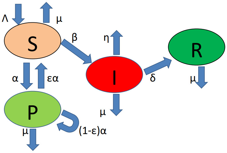
In the case of an epidemic, the government (or population itself) can use protection for reducing the epidemic. This research investigates the global dynamics of a delayed epidemic model with partial susceptible protection. A threshold dynamics is obtained in terms of the basic reproduction number, where for $ R_0 < 1 $ the infection will extinct from the population. But, for $ R_0 > 1 $ it has been shown that the disease will persist, and the unique positive equilibrium is globally asymptotically stable. The principal purpose of this research is to determine a relation between the isolation rate and the basic reproduction number in such a way we can eliminate the infection from the population. Moreover, we will determine the minimal protection force to eliminate the infection for the population. A comparative analysis with the classical SIR model is provided. The results are supported by some numerical illustrations with their epidemiological relevance.

| [1] | Ebola (maladie a virus), https://www.who.int/fr/news-room/fact-sheets/detail/ebola-virus-disease. |
| [2] | H. T. Abdoul-Azize, R. El Gamil, Social Protection as a Key Tool in Crisis Management: Learnt Lessons from the COVID-19 Pandemic, Glob. Soc. Welf., 8 (2021), 107–116. doi: 10.1007/s40609-020-00190-4 |
| [3] | S. Bentout, A. Tridane, S. Djilali, T. M. Touaoula, Age-Structured Modeling of COVID-19 Epidemic in the USA, UAE and Algeria, Alex Eng. J., 60 (2021), 401–411. https://doi.org/10.1016/j.aej.2020.08.053 |
| [4] | S. Djilali, L. Benahmadi, A. Tridane, K. Niri, Modeling the Impact of Unreported Cases of the COVID-19 in the North African Countries, Biology, 9 (2020), 373. https://doi.org/10.3390/biology9110373 |
| [5] | P. C. Jentsch, M. Anand, C. T. Bauch, Prioritising COVID-19 vaccination in changing social and epidemiological landscapes: A mathematical modelling study, Lan. Inf. Dis., (2021). DOI: 10.1016/S1473-3099(21)00057-8. |
| [6] | A.Zeb, E. Alzahrani, V. S. Erturk, G. Zaman, Mathematical Model for Coronavirus Disease 2019 (COVID-19) Containing Isolation Class, Bio. Med. Res. Int., 2000 (2020). https://doi.org/10.1155/2020/3452402 |
| [7] | Z. Zhang, A. Zeb, E. Alzahrani, S. Iqbal, Crowding effects on the dynamics of COVID-19 mathematical model, Adv. Differ. Equ., 1 (2020), 1–13. https://doi.org/10.1186/s13662-020-03137-3 |
| [8] | S. Bushnaq, T. Saeed, D. F. M. Torres, A. Zeb, Control of COVID-19 dynamics through a fractional-order model, Alex. Eng. J., 60 (2021), 3587–3592. https://doi.org/10.1016/j.aej.2021.02.022 |
| [9] | S. Djilali, S. Bentout, Global dynamics of SVIR epidemic model with distributed delay and imperfect vaccine, Res. Phy., 25 (2021), 104245.https://doi.org/10.1016/j.rinp.2021.104245 |
| [10] | X. Duan, S. Yuan, X. Li, Global stability of an SVIR model with age of vaccination, App. Math. Comp., 226 (2014), 528–540. https://doi.org/10.1016/j.camwa.2014.06.002 |
| [11] | C. Zhang, J. Gao, H. Sun, J. Wang, Dynamics of a reaction-diffusion SVIR model in a spatial heterogeneous environment, Phy. A., 533 (2019) 122049.DOI: 10.1016/j.physa.2019.122049 |
| [12] | X. Zhang, Q. Yang, Threshold behavior in a stochastic SVIR model with general incidence rates, Appl. Math. Lett., 121 (2021), 107403.DOI: 10.1016/j.aml.2021.107403 |
| [13] | M. Adimy, A. Chekroun, C. P. Ferreira, Global dynamics of a differential-difference system: A case of Kermack-McKendrick SIR model with age-structured protection phase, Math. Biosci. Eng., 17 (2020), 1329–1354. doi: 10.3934/mbe.2020067 |
| [14] | E. Beretta, Y. Takeuchi, Global stability of an SIR epidemic model with time delays, J. Math. Biol., 33 (1995), 250–260. https://doi.org/10.1007/BF00169563 |
| [15] | E. Beretta, T. Hara, W. Ma, Y. Takeuchi, Global asymptotic stability of an SIR epidemic model with distributed time delay, Non. Ana. Theo. Meth. Appl., 47 (2001), 4107–4115. DOI: 10.1016/S0362-546X(01)00528-4 |
| [16] | G. Huang, A. Liu, A note on global stability for a heroin epidemic model with distributed delay, Appl. Math. Let., 26 (2013), 687–691. https://doi.org/10.1016/j.aml.2013.01.010 |
| [17] | C. McCluskey, Complete global stability for an SIR epidemic model with delay-Distributed or discrete, Non. Anal. Re. Worl. Appl., 11 (2010), 55–59. https://doi.org/10.1016/j.nonrwa.2008.10.014 |
| [18] | G. Huang, A. Liu, A note on global stability for a heroin epidemic model with distributed delay, Appl. Math. Let., 26 (2013), 687–691. https://doi.org/10.1016/j.aml.2013.01.010 |
| [19] | J. Belair, Stability in a model of a delayed neural network, J. Dyn. Diff. Equ., 5 (1993), 607–623. https://doi.org/10.1007/BF01049141 |


Figures(6)

Abdelheq Mezouaghi, Salih Djillali, Anwar Zeb, Kottakkaran Sooppy Nisar. Global proprieties of a delayed epidemic model with partial susceptible protection[J]. Mathematical Biosciences and Engineering, 2022, 19(1): 209-224. doi: 10.3934/mbe.2022011


 DownLoad: