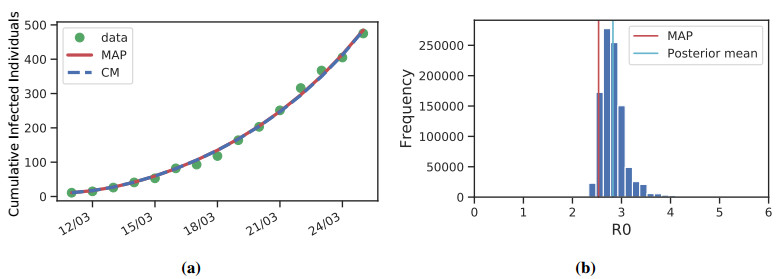
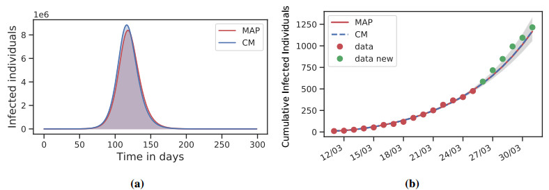
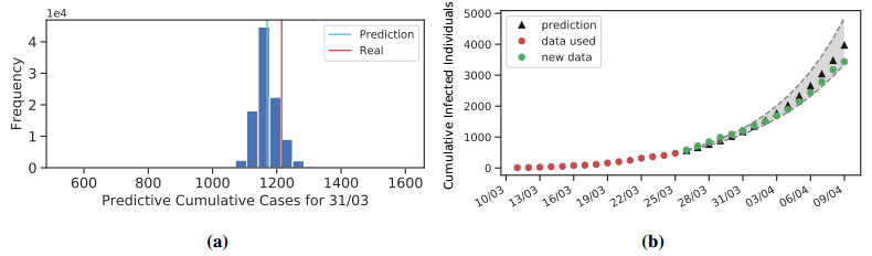
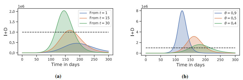
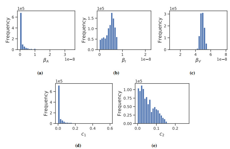
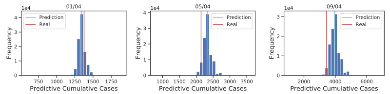
In this paper we develop a compartmental epidemic model to study the transmission dynamics of the COVID-19 epidemic outbreak, with Mexico as a practical example. In particular, we evaluate the theoretical impact of plausible control interventions such as home quarantine, social distancing, cautious behavior and other self-imposed measures. We also investigate the impact of environmental cleaning and disinfection, and government-imposed isolation of infected individuals. We use a Bayesian approach and officially published data to estimate some of the model parameters, including the basic reproduction number. Our findings suggest that social distancing and quarantine are the winning strategies to reduce the impact of the outbreak. Environmental cleaning can also be relevant, but its cost and effort required to bring the maximum of the outbreak under control indicate that its cost-efficacy is low.
Citation: Fernando Saldaña, Hugo Flores-Arguedas, José Ariel Camacho-Gutiérrez, Ignacio Barradas. Modeling the transmission dynamics and the impact of the control interventions for the COVID-19 epidemic outbreak[J]. Mathematical Biosciences and Engineering, 2020, 17(4): 4165-4183. doi: 10.3934/mbe.2020231
In this paper we develop a compartmental epidemic model to study the transmission dynamics of the COVID-19 epidemic outbreak, with Mexico as a practical example. In particular, we evaluate the theoretical impact of plausible control interventions such as home quarantine, social distancing, cautious behavior and other self-imposed measures. We also investigate the impact of environmental cleaning and disinfection, and government-imposed isolation of infected individuals. We use a Bayesian approach and officially published data to estimate some of the model parameters, including the basic reproduction number. Our findings suggest that social distancing and quarantine are the winning strategies to reduce the impact of the outbreak. Environmental cleaning can also be relevant, but its cost and effort required to bring the maximum of the outbreak under control indicate that its cost-efficacy is low.

| [1] | H. A. Rothan, S. N. Byrareddy, The epidemiology and pathogenesis of coronavirus disease (COVID-19) outbreak, J. Autoimmun., (2020), 102433. |
| [2] | World Health Organization, Coronavirus disease 2019 (COVID-19): situation report-51, 2020. Available from: https://www.who.int/docs/default-source/coronaviruse/situationreports/20200311-sitrep-51-COVID-19.pdf. |
| [3] | World Health Organization, Assessment of risk factors for coronavirus disease 2019 (COVID-19) in health workers: protocol for a case-control study, 26 May 2020. Available from: https://www.who.int/publications/i/item/assessment-of-risk-factors-for-coronavirus-disease-2019-(COVID-19)-in-health-workers-protocol-for-a-case-control-study |
| [4] | A. Teslya, T. M. Pham, N. E. Godijk, M. E. Kretzschmar, M. C. Bootsma, G. Rozhnova, Impact of self-imposed prevention measures and short-term government intervention on mitigating and delaying a COVID-19 epidemic, medRxiv, (2020), 2020.03.12.20034827. |
| [5] | F. Brauer, Mathematical epidemiology: Past, present, and future, Infect. Dis. Model., 2 (2017), 113-127. |
| [6] | J. Jia, J. Ding, S. Liu, G. Liao, J. Li, B. Duan, et al., Modeling the control of COVID-19: Impact of policy interventions and meteorological factors, arXiv, (2020), 2003.02985. |
| [7] | S. S. Nadim, I. Ghosh, J. Chattopadhyay, Short-term predictions and prevention strategies for COVID-2019: A model based study, arXiv, (2020), 2003.08150. |
| [8] | B. Tang, X. Wang, Q. Li, N. L. Bragazzi, S. Tang, Y. Xiao, et al., Estimation of the transmission risk of the 2019-ncov and its implication for public health interventions, J. Clin. Med., 9 (2020), 462. |
| [9] |
C. Yang, J. Wang, A mathematical model for the novel coronavirus epidemic in Wuhan, China, Math. Biosci. Eng., 17 (2020), 2708-2724. doi: 10.3934/mbe.2020148

|
| [10] | Y. Liu, A. A. Gayle, A. Wilder-Smith, J. Rocklöv, The reproductive number of COVID-19 is higher compared to SARS coronavirus, J. Travel. Med., 27 (2020), taaa021. |
| [11] |
G. Kampf, D. Todt, S. Pfaender, E. Steinmann, Persistence of coronaviruses on inanimate surfaces and their inactivation with biocidal agents, J. Hosp. Infect., 104 (2020), 246-251. doi: 10.1016/j.jhin.2020.01.022
|
| [12] | H. W. Hethcote, The mathematics of infectious diseases, SIAM Rev. Soc. Ind. Appl. Math., 42 (2000), 599-653. |
| [13] | O. Diekmann, J. A. P. Heesterbeek, J. A. Metz, On the definition and the computation of the basic reproduction ratio r 0 in models for infectious diseases in heterogeneous populations, J. Math. Biol., 28 (1990), 365-382. |
| [14] |
P. Van den Driessche, J. Watmough, Reproduction numbers and sub-threshold endemic equilibria for compartmental models of disease transmission, Math. Biosci., 180 (2002), 29-48. doi: 10.1016/S0025-5564(02)00108-6
|
| [15] | J. A. Backer, D. Klinkenberg, J. Wallinga, Incubation period of 2019 novel coronavirus (2019-ncov) infections among travellers from Wuhan, China, 20-28 january 2020, Euro. Surveil., 25 (2020), 2000062. |
| [16] | Secretary of Health, Aviso epidemiológico: casos de infección respiratoria asociados a nuevo-coronavirus-2019-ncov, 2020. Available from: https://www.gob.mx/salud/documentos/avisoepidemiologico-casos-de-infeccion-respiratoria-asociados-a-nuevo-coronavirus-2019-ncov. |
| [17] |
J. A. Christen, C. Fox, A general purpose sampling algorithm for continuous distributions (the t-walk), Bayesian Anal., 5 (2010), 263-281. doi: 10.1214/10-BA603
|
| [18] | El Financiero, Al 10% de los casos sospechosos de COVID-19 con síntomas leves se les aplica prueba: Imss, 2020. Available from: https://www.elfinanciero.com.mx/nacional/al-10-de-loscasos-sospechosos-de-covid-19-con-sintomas-leves-se-les-aplica-prueba-imss. |
| [19] |
E. Shim, A. Tariq, W. Choi, Y. Lee, G. Chowell, Transmission potential and severity of COVID-19 in South Korea, Int. J. Infect. Dis., 93 (2020), 339-344. doi: 10.1016/j.ijid.2020.03.031
|
| [20] | A. Kuzdeuov, D. Baimukashev, A. Karabay, B. Ibragimov, A. Mirzakhmetov, M. Nurpeiissov, et al., A network-based stochastic epidemic simulator: Controlling COVID-19 with region-specific policies, medRxiv, (2020), 2020.05.02.20089136v1. |
| [21] | J. Herman, W. Usher, SALib: An open-source python library for sensitivity analysis, J. Open Res. Softw., 2 (2017), 97. |
Figures(10) / Tables(1)

Fernando Saldaña, Hugo Flores-Arguedas, José Ariel Camacho-Gutiérrez, Ignacio Barradas. Modeling the transmission dynamics and the impact of the control interventions for the COVID-19 epidemic outbreak[J]. Mathematical Biosciences and Engineering, 2020, 17(4): 4165-4183. doi: 10.3934/mbe.2020231


 DownLoad: