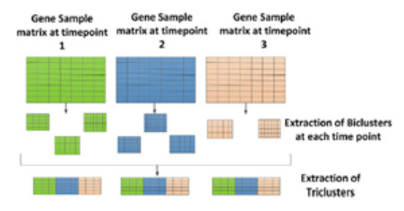
HIV-1 is a virus that destroys CD4 + cells in the body's immune system, causing a drastic decline in immune system performance. Analysis of HIV-1 gene expression data is urgently needed. Microarray technology is used to analyze gene expression data by measuring the expression of thousands of genes in various conditions. The gene expression series data, which are formed in three dimensions, are analyzed using triclustering. Triclustering is an analysis technique for 3D data that aims to group data simultaneously into rows and columns across different times/conditions. The result of this technique is called a tricluster. A tricluster is a subspace in the form of a subset of rows, columns, and time/conditions. In this study, we used the $ \delta $-Trimax, THD Tricluster, and MOEA methods by applying different measures, namely, transposed virtual error, the New Residue Score, and the Multi Slope Measure. The gene expression data consisted of 22,283 probe gene IDs, 40 observations, and four conditions: normal, acute, chronic, and non-progressor. Tricluster evaluation was carried out based on intertemporal homogeneity. An analysis of the probe ID gene that affects AIDS was carried out through this triclustering process. Based on this analysis, a gene symbol which is biomarkers associated with AIDS due to HIV-1, HLA-C, was found in every condition for normal, acute, chronic, and non-progressive HIV-1 patients.
Citation: Titin Siswantining, Alhadi Bustamam, Devvi Sarwinda, Saskya Mary Soemartojo, Moh. Abdul Latief, Elke Annisa Octaria, Anggrainy Togi Marito Siregar, Oon Septa, Herley Shaori Al-Ash, Noval Saputra. Triclustering method for finding biomarkers in human immunodeficiency virus-1 gene expression data[J]. Mathematical Biosciences and Engineering, 2022, 19(7): 6743-6763. doi: 10.3934/mbe.2022318
HIV-1 is a virus that destroys CD4 + cells in the body's immune system, causing a drastic decline in immune system performance. Analysis of HIV-1 gene expression data is urgently needed. Microarray technology is used to analyze gene expression data by measuring the expression of thousands of genes in various conditions. The gene expression series data, which are formed in three dimensions, are analyzed using triclustering. Triclustering is an analysis technique for 3D data that aims to group data simultaneously into rows and columns across different times/conditions. The result of this technique is called a tricluster. A tricluster is a subspace in the form of a subset of rows, columns, and time/conditions. In this study, we used the $ \delta $-Trimax, THD Tricluster, and MOEA methods by applying different measures, namely, transposed virtual error, the New Residue Score, and the Multi Slope Measure. The gene expression data consisted of 22,283 probe gene IDs, 40 observations, and four conditions: normal, acute, chronic, and non-progressor. Tricluster evaluation was carried out based on intertemporal homogeneity. An analysis of the probe ID gene that affects AIDS was carried out through this triclustering process. Based on this analysis, a gene symbol which is biomarkers associated with AIDS due to HIV-1, HLA-C, was found in every condition for normal, acute, chronic, and non-progressive HIV-1 patients.

| [1] | G. Ardaneswari, A. Bustamam, T. Siswantining, Implementation of parallel k-means algorithm for two-phase method biclustering in carcinoma tumor gene expression data, in AIP Conference Proceedings, 1825 (2017). https://doi.org/10.1063/1.4978973 |
| [2] |
T. Siswantining, N. P. Purwandani, M. Susilowati, A. Wibowo, Geoinformatics of tuberculosis (TB) disease in Jakarta city Indonesia, GEOMATE J., 19 (2020), 35–42. https://doi.org/10.21660/2020.72.5599 doi: 10.21660/2020.72.5599

|
| [3] | M. A. Latief, A. Bustamam, T. Siswantining, Performance evaluation xgboost in handling missing value on classification of hepatocellular carcinoma gene expression data, in 2020 4th International Conference on Informatics and Computational Sciences (ICICoS), (2020), 1–6. |
| [4] | T. Siswantining, T. Anwar, D. Sarwinda, H. Al-Ash, A novel centroid initialization in missing value imputation towards mixed datasets, Commun. Math. Biol. Neurosci., 2021 (2021). https://doi.org/10.28919/cmbn/5344 |
| [5] | M. A. Latief, T. Siswantining, A. Bustamam, D. Sarwinda, A comparative performance evaluation of random forest feature selection on classification of hepatocellular carcinoma gene expression data, in 2019 3rd International Conference on Informatics and Computational Sciences (ICICoS), (2019), 1–6. |
| [6] | D. A. Apriana, T. Siswantining, D. Sarwinda, S. M. Soemartojo, Triclustering analysis using extended dimension iterative signature algorithm (edisa) on lung disease gene expression data, in 2020 3rd International Conference on Biomedical Engineering (IBIOMED), IEEE, (2020), 7–12. |
| [7] | I. M. Sari, S. M. Soemartojo, T. Siswantining, D. Sarwinda, Mining biological information from 3d medulloblastoma cancerous gene expression data using timesvector triclustering method, in 2020 4th International Conference on Informatics and Computational Sciences (ICICoS), (2020), 1–6. |
| [8] |
A. Bustamam, T. Siswantining, T. P. Kaloka, O. Swasti, Application of BiMax, POLS, and LCM-MBC to find bicluster on interactions protein between HIV-1 and human, Austrian J. Stat., 49 (2020), 1–18. https://doi.org/10.17713/ajs.v49i3.1011 doi: 10.17713/ajs.v49i3.1011
|
| [9] |
O. Alter, G. H. Golub, Singular value decomposition of genome-scale mrna lengths distribution reveals asymmetry in rna gel electrophoresis band broadening, Proc. Natl. Acad. Sci., 103 (2006), 11828–11833. https://doi.org/10.1073/pnas.0604756103 doi: 10.1073/pnas.0604756103
|
| [10] |
T. Siswantining, N. Saputra, D. Sarwinda, H. S. Al-Ash, Triclustering discovery using the $\delta$-trimax method on microarray gene expression data, Symmetry, 13 (2021), 437. https://doi.org/10.3390/sym13030437 doi: 10.3390/sym13030437
|
| [11] | H. Ahmed, P. Mahanta, D. Bhattacharyya, J. Kalita, A. Ghosh, Intersected coexpressed subcube miner: An effective triclustering algorithm, in 2011 World Congress on Information and Communication Technologies, IEEE, (2011), 846–851. |
| [12] | P. S. Mahiskar, A. Bhade, P. Chatur, The data mining triclustering algorithm for mining real valued datasets-a review, Int. J. Comput. Sci. Eng. Technol., 2 (2012). |
| [13] | A. Rachma, S. Soemartojo, T. Siswantining, Thd-tricluster method on gene expression data of multiple sclerosis patients receiving interferon-beta therapy, in AIP Conference Proceedings, 2374 (2021), 030002. https://doi.org/10.1063/5.0058711 |
| [14] | E. A. Octaria, T. Siswantining, A. Bustamam, D. Sarwinda, Kernel PCA and SVM-RFE based feature selection for classification of dengue microarray dataset, in AIP Conference Proceedings, 2264 (2020), 03004. https://doi.org/10.1063/5.0023930 |
| [15] | A. T. M. Siregar, T. Siswantining, A. Bustamam, D. Sarwinda, Comparison of supervised models in hepatocellular carcinoma tumor classification based on expression data using principal component analysis (PCA), in AIP Conference Proceedings, 2264 (2020), 030002. https://doi.org/10.1063/5.0023931 |
| [16] | W. H. Yang, D. Q. Dai, H. Yan, Finding correlated biclusters from gene expression data, IEEE Trans. Knowl. Data Eng., 23 (2011), 568–584. |
| [17] |
A. Trkola, Hiv–host interactions: vital to the virus and key to its inhibition, Curr. Opin. Microbiol., 7 (2004), 407–411. https://doi.org/10.1016/j.mib.2004.06.002 doi: 10.1016/j.mib.2004.06.002
|
| [18] |
D. Gutiérrez-Avilés, C. Rubio-Escudero, F. Martínez-Álvarez, J. C. Riquelme, TriGen: A genetic algorithm to mine triclusters in temporal gene expression data, Neurocomputing, 132 (2014), 42–53. https://doi.org/10.1016/j.neucom.2013.03.061 doi: 10.1016/j.neucom.2013.03.061
|
| [19] |
T. Kakati, H. A. Ahmed, D. K. Bhattacharyya, J. K. Kalita, Thd-tricluster: A robust triclustering technique and its application in condition specific change analysis in hiv-1 progression data, Comput. Biol. Chem., 75 (2018), 154–167. https://doi.org/10.1016/j.compbiolchem.2018.05.007 doi: 10.1016/j.compbiolchem.2018.05.007
|
| [20] | Y. Cheng, G. M. Church, Biclustering of expression data, in Ismb, 8 (2000), 93–103. |
| [21] |
A. Bustamam, S. Formalidin, T. Siswantining, Z. Rustam, Finding correlated biclusters from microarray data using the modified lift algorithm based on new residue score, Int. J. Data Min. Bioinf., 24 (2020), 326. https://doi.org/10.1504/ijdmb.2020.113691 doi: 10.1504/ijdmb.2020.113691
|
| [22] |
B. Pontes, R. Girldez, J. S. Aguilar-Ruiz, Quality measures for gene expression biclusters, PloS One, 10 (2015), e0115497. https://doi.org/10.1371/journal.pone.0115497 doi: 10.1371/journal.pone.0115497
|
| [23] | D. Gutiérrez-Avilés, C. Rubio-Escudero, MSL: a measure to evaluate three-dimensional patterns in gene expression data, Evol. Bioinf., 11 (2015), EBO-S25822. https://journals.sagepub.com/doi/full/10.4137/EBO.S25822 |


Figures(7) / Tables(8)

Titin Siswantining, Alhadi Bustamam, Devvi Sarwinda, Saskya Mary Soemartojo, Moh. Abdul Latief, Elke Annisa Octaria, Anggrainy Togi Marito Siregar, Oon Septa, Herley Shaori Al-Ash, Noval Saputra. Triclustering method for finding biomarkers in human immunodeficiency virus-1 gene expression data[J]. Mathematical Biosciences and Engineering, 2022, 19(7): 6743-6763. doi: 10.3934/mbe.2022318


 DownLoad: