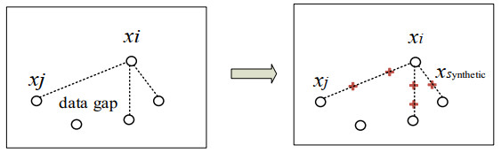
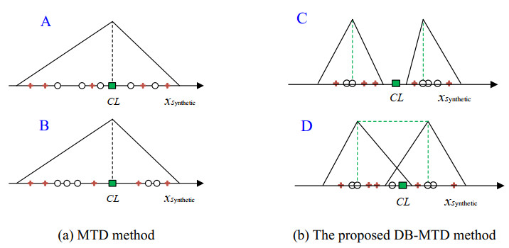
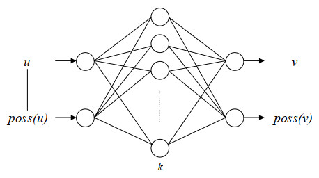
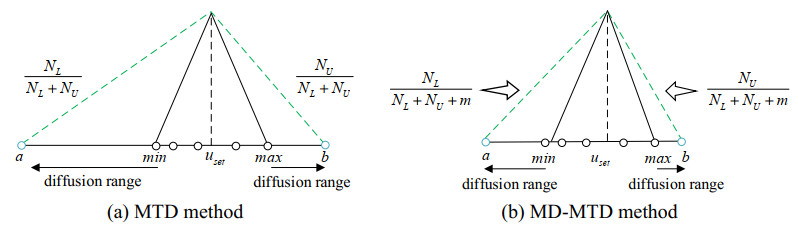
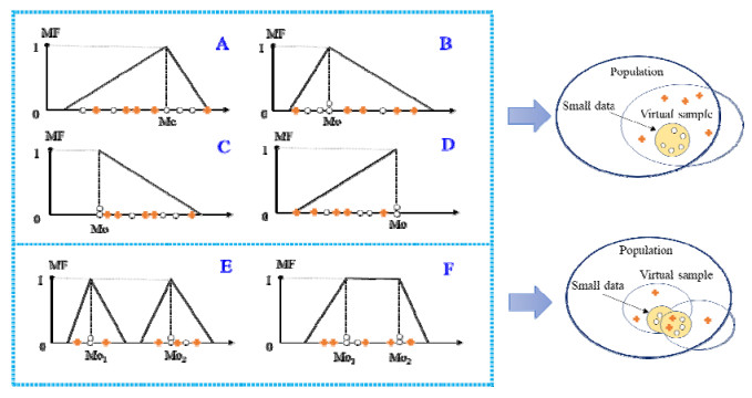
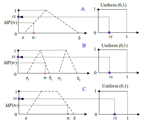
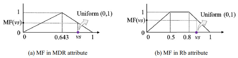
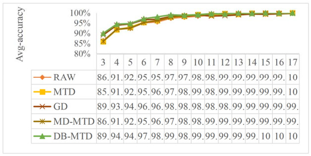
In the medical field, researchers are often unable to obtain the sufficient samples in a short period of time necessary to build a stable data-driven forecasting model used to classify a new disease. To address the problem of small data learning, many studies have demonstrated that generating virtual samples intended to augment the amount of training data is an effective approach, as it helps to improve forecasting models with small datasets. One of the most popular methods used in these studies is the mega-trend-diffusion (MTD) technique, which is widely used in various fields. The effectiveness of the MTD technique depends on the degree of data diffusion. However, data diffusion is seriously affected by extreme values. In addition, the MTD method only considers data fitted using a unimodal triangular membership function. However, in fact, data may come from multiple distributions in the real world. Therefore, considering the fact that data comes from multi-distributions, in this paper, a distance-based mega-trend-diffusion (DB-MTD) technique is proposed to appropriately estimate the degree of data diffusion with less impacts from extreme values. In the proposed method, it is assumed that the data is fitted by the triangular and trapezoidal membership functions to generate virtual samples. In addition, a possibility evaluation mechanism is proposed to measure the applicability of the virtual samples. In our experiment, two bladder cancer datasets are used to verify the effectiveness of the proposed DB-MTD method. The experimental results demonstrated that the proposed method outperforms other VSG techniques in classification and regression items for small bladder cancer datasets.
Citation: Liang-Sian Lin, Susan C Hu, Yao-San Lin, Der-Chiang Li, Liang-Ren Siao. A new approach to generating virtual samples to enhance classification accuracy with small data—a case of bladder cancer[J]. Mathematical Biosciences and Engineering, 2022, 19(6): 6204-6233. doi: 10.3934/mbe.2022290
In the medical field, researchers are often unable to obtain the sufficient samples in a short period of time necessary to build a stable data-driven forecasting model used to classify a new disease. To address the problem of small data learning, many studies have demonstrated that generating virtual samples intended to augment the amount of training data is an effective approach, as it helps to improve forecasting models with small datasets. One of the most popular methods used in these studies is the mega-trend-diffusion (MTD) technique, which is widely used in various fields. The effectiveness of the MTD technique depends on the degree of data diffusion. However, data diffusion is seriously affected by extreme values. In addition, the MTD method only considers data fitted using a unimodal triangular membership function. However, in fact, data may come from multiple distributions in the real world. Therefore, considering the fact that data comes from multi-distributions, in this paper, a distance-based mega-trend-diffusion (DB-MTD) technique is proposed to appropriately estimate the degree of data diffusion with less impacts from extreme values. In the proposed method, it is assumed that the data is fitted by the triangular and trapezoidal membership functions to generate virtual samples. In addition, a possibility evaluation mechanism is proposed to measure the applicability of the virtual samples. In our experiment, two bladder cancer datasets are used to verify the effectiveness of the proposed DB-MTD method. The experimental results demonstrated that the proposed method outperforms other VSG techniques in classification and regression items for small bladder cancer datasets.

| [1] |
P. Gontero, A. Tizzani, G. H. Muir, E. Caldarera, M. Pavone Macaluso, The genetic alterations in the oncogenic pathway of transitional cell carcinoma of the bladder and its prognostic value, Urol. Res., 29 (2001), 377–387. https://doi.org/10.1007/s002400100216 doi: 10.1007/s002400100216

|
| [2] |
V. Tut, K. Braithwaite, B. Angus, D. Neal, J. Lunec, J. Mellon, Cyclin D1 expression in transitional cell carcinoma of the bladder: correlation with p53, waf1, pRb and Ki67, Br. J. Cancer, 84 (2001), 270–275. https://doi.org/10.1054/bjoc.2000.1557 doi: 10.1054/bjoc.2000.1557
|
| [3] |
A. Colquhoun, S. Sundar, P. Rajjayabun, T. Griffiths, R. Symonds, J. Mellon, Epidermal growth factor receptor status predicts local response to radical radiotherapy in muscle-invasive bladder cancer, Clin. Oncol., 18 (2006), 702–709. https://doi.org/10.1016/j.clon.2006.08.003 doi: 10.1016/j.clon.2006.08.003
|
| [4] |
P. Luukka, Similarity classifier in diagnosis of bladder cancer, Comput. Methods Programs Biomed., 89 (2008), 43–49. https://doi.org/10.1016/j.cmpb.2007.10.001 doi: 10.1016/j.cmpb.2007.10.001
|
| [5] |
G. Y. Chao, T. I. Tsai, T. J. Lu, H. C. Hsu, B. Y. Bao, W. Y. Wu, et al, A new approach to prediction of radiotherapy of bladder cancer cells in small dataset analysis, Expert Syst. Appl., 38 (2011), 7963–7969. https://doi.org/10.1016/j.eswa.2010.12.035 doi: 10.1016/j.eswa.2010.12.035
|
| [6] |
T. W. Liao, Diagnosis of bladder cancers with small sample size via feature selection, Expert Syst. Appl., 38 (2011), 4649–4654. https://doi.org/10.1016/j.eswa.2010.09.135 doi: 10.1016/j.eswa.2010.09.135
|
| [7] |
T. I. Tsai, Y. Zhang, Z. Zhang, G. Y. Chao, C. C. Tsai, Considering relationship of proteins for radiotherapy prognosis of bladder cancer cells in small data set, Methods Inf. Med., 57 (2018), 220–229. https://doi.org/10.3414/ME17-02-0003 doi: 10.3414/ME17-02-0003
|
| [8] |
M. D. Robinson, G. K. Smyth, Small-sample estimation of negative binomial dispersion, with applications to SAGE data, Biostatistics, 9 (2008), 321–332. https://doi.org/10.1093/biostatistics/kxm030 doi: 10.1093/biostatistics/kxm030
|
| [9] |
S. Lee, M. J. Emond, M. J. Bamshad, K. C. Barnes, M. J. Rieder, D. A. Nickerson, et al., Optimal unified approach for rare-variant association testing with application to small-sample case-control whole-exome sequencing studies, Am. J. Hum. Genet., 91 (2012), 224–237. https://doi.org/10.1016/j.ajhg.2012.06.007 doi: 10.1016/j.ajhg.2012.06.007
|
| [10] |
Y. Zhao, N. J. Fesharaki, H. Liu, J. Luo, Using data-driven sublanguage pattern mining to induce knowledge models: application in medical image reports knowledge representation, BMC Med. Inf. Decis. Making, 18 (2018), 1–13. https://doi.org/10.1186/s12911-018-0645-3 doi: 10.1186/s12911-017-0580-8
|
| [11] |
L. Stainier, A. Leygue, M. Ortiz, Model-free data-driven methods in mechanics: material data identification and solvers, Comput. Mech., 64 (2019), 381–393. https://doi.org/10.1007/s00466-019-01731-1 doi: 10.1007/s00466-019-01731-1
|
| [12] |
E. Ntoutsi, P. Fafalios, U. Gadiraju, V. Iosifidis, W. Nejdl, M. E. Vidal, et al., Bias in data‐driven artificial intelligence systems—An introductory survey, Wiley Interdiscip. Rev.: Data Min. Knowl. Discovery, 10 (2020), e1356. https://doi.org/10.1002/widm.1356 doi: 10.1002/widm.1356
|
| [13] |
T. Mao, L. Yu, Y. Zhang, L. Zhou, Modified Mahalanobis-Taguchi System based on proper orthogonal decomposition for high-dimensional-small-sample-size data classification, Math. Biosci. Eng., 18 (2020), 426–444. https://doi.org/10.3934/mbe.2021023 doi: 10.3934/mbe.2021023
|
| [14] |
I. Izonin, R. Tkachenko, I. Dronyuk, P. Tkachenko, M. Gregus, M. Rashkevych, Predictive modeling based on small data in clinical medicine: RBF-based additive input-doubling method, Math. Biosci. Eng., 18 (2021), 2599–2613. https://doi.org/10.3934/mbe.2020392 doi: 10.3934/mbe.2021132
|
| [15] |
Y. Liu, Y. Zhou, X. Liu, F. Dong, C. Wang, Z. Wang, Wasserstein GAN-based small-sample augmentation for new-generation artificial intelligence: a case study of cancer-staging data in biology, Engineering, 5 (2019), 156–163. https://doi.org/10.1016/j.eng.2018.11.018 doi: 10.1016/j.eng.2018.11.018
|
| [16] |
H. Han, M. Zhou, Y. Zhang, Can virtual samples solve small sample size problem of KISSME in pedestrian re-identification of smart transportation?, IEEE Trans. Intell. Transp. Syst., 21 (2020), 3766–3776. https://doi.org/10.1109/TITS.2019.2933509 doi: 10.1109/TITS.2019.2933509
|
| [17] |
Z. Liu, Y. Li, Small data-driven modeling of forming force in single point incremental forming using neural networks, Eng. Comput., 36 (2020), 1589–1597. https://doi.org/10.1007/s00366-019-00781-6 doi: 10.1007/s00366-019-00781-6
|
| [18] |
Q. X. Zhu, Z. S. Chen, X. H. Zhang, A. Rajabifard, Y. Xu, Y. Q. Chen, Dealing with small sample size problems in process industry using virtual sample generation: a Kriging-based approach, Soft Comput., 24 (2020), 6889–6902. https://doi.org/10.1007/s00500-019-04326-3 doi: 10.1007/s00500-019-04326-3
|
| [19] |
N. V. Chawla, K. W. Bowyer, L. O. Hall, W. P. Kegelmeyer, SMOTE: synthetic minority over-sampling technique, J. Artif. Intell. Res., 16 (2002), 321–357. https://doi.org/10.1613/jair.953 doi: 10.1613/jair.953
|
| [20] | B. Efron, R. LePage, Introduction to Bootstrap, Wiley & Sons, New York, 1992. |
| [21] |
S. Lee, A. Ahmad, G. Jeon, Combining bootstrap aggregation with support vector regression for small blood pressure measurement, J. Med. Syst., 42 (2018), 1–7. https://doi.org/10.1007/s10916-018-0913-x doi: 10.1007/s10916-017-0844-y
|
| [22] |
M. F. Ijaz, M. Attique, Y. Son, Data-driven cervical cancer prediction model with outlier detection and over-sampling methods, Sensors, 20 (2020), 2809. https://doi.org/10.3390/s20102809 doi: 10.3390/s20102809
|
| [23] |
M. La Rocca, C. Perna, Nonlinear autoregressive sieve bootstrap based on extreme learning machines, Math. Biosci. Eng., 17 (2020), 636–653. https://doi.org/10.3934/mbe.202003 doi: 10.3934/mbe.2020033
|
| [24] |
S. Cho, M. Jang, S. Chang, Virtual sample generation using a population of networks, Neural Process Lett., 5 (1997), 21–27. https://doi.org/10.1023/A:1009653706403 doi: 10.1023/A:1009653706403
|
| [25] |
C. Huang, C. Moraga, A diffusion-neural-network for learning from small samples, Int. J. Approx. Reasoning, 35 (2004), 137–161. https://doi.org/10.1016/j.ijar.2003.06.001 doi: 10.1016/j.ijar.2003.06.001
|
| [26] | I. Goodfellow, J. Pouget-Abadie, M. Mirza, B. Xu, D. Warde-Farley, S. Ozair, et al., Generative adversarial nets, in Proceedings of the International Conference on Neural Information Processing Systems (NIPS), (2014), 2672–2680. |
| [27] |
X. H. Zhang, Y. Xu, Y. L. He, Q. X. Zhu, Novel manifold learning based virtual sample generation for optimizing soft sensor with small data, ISA Trans., 109 (2021), 229–241. https://doi.org/10.1016/j.isatra.2020.10.006 doi: 10.1016/j.isatra.2020.10.006
|
| [28] |
D. C. Li, C. S. Wu, T. I. Tsai, Y. S. Lina, Using mega-trend-diffusion and artificial samples in small data set learning for early flexible manufacturing system scheduling knowledge, Comput. Oper. Res., 34 (2007), 966–982. https://doi.org/10.1016/j.cor.2005.05.019 doi: 10.1016/j.cor.2005.05.019
|
| [29] |
M. R. Rahimi, H. Karimi, F. Yousefi, Prediction of carbon dioxide diffusivity in biodegradable polymers using diffusion neural network, Heat Mass Transfer, 48 (2012), 1357–1365. https://doi.org/10.1007/s00231-012-0982-1 doi: 10.1007/s00231-012-0982-1
|
| [30] |
A. Majid, S. Ali, M. Iqbal, N. Kausar, Prediction of human breast and colon cancers from imbalanced data using nearest neighbor and support vector machines, Comput. Methods Programs Biomed., 113 (2014), 792–808. https://doi.org/10.1016/j.cmpb.2014.01.001 doi: 10.1016/j.cmpb.2014.01.001
|
| [31] |
B. Zhu, Z. Chen, L. Yu, A novel mega-trend-diffusion for small sample, CIESC J., 67 (2016), 820–826. https://doi.org/10.11949/j.issn.0438-1157.20151921 doi: 10.11949/j.issn.0438-1157.20151921
|
| [32] |
L. Yu, X. Zhang, Can small sample dataset be used for efficient internet loan credit risk assessment? Evidence from online peer to peer lending, Finance Res. Lett., 38 (2021), 101521. https://doi.org/10.1016/j.frl.2020.101521 doi: 10.1016/j.frl.2020.101521
|
| [33] |
J. Yang, X. Yu, Z. Q. Xie, J. P. Zhang, A novel virtual sample generation method based on Gaussian distribution, Knowl. Based. Syst., 24 (2011), 740–748. https://doi.org/10.1016/j.knosys.2010.12.010 doi: 10.1016/j.knosys.2010.12.010
|
| [34] |
K. Wang, J. Li, F. Tsung, Distribution inference from early-stage stationary data streams by transfer learning, ⅡSE Trans., (2021), 1–25. https://doi.org/10.1080/24725854.2021.1875520 doi: 10.1080/24725854.2021.1875520
|
| [35] |
O. Troyanskaya, M. Cantor, G. Sherlock, P. Brown, T. Hastie, R. Tibshirani, et al., Missing value estimation methods for DNA microarrays, Bioinformatics, 17 (2001), 520–525. https://doi.org/10.1093/bioinformatics/17.6.520 doi: 10.1093/bioinformatics/17.6.520
|
| [36] |
G. E. Batista, M. C. Monard, An analysis of four missing data treatment methods for supervised learning, Appl. Artif. Intell., 17 (2003), 519–533. https://doi.org/10.1080/713827181 doi: 10.1080/713827181
|
| [37] |
D. V. Nguyen, N. Wang, R. J. Carroll, Evaluation of missing value estimation for microarray data, Data Sci. J., 2 (2004), 347–370. https://doi.org/10.6339/JDS.2004.02(4).170 doi: 10.6339/JDS.2004.02(4).170
|
| [38] |
A. Jadhav, D. Pramod, K. Ramanathan, Comparison of performance of data imputation methods for numeric dataset, Appl. Artif. Intell., 33 (2019), 913–933. https://doi.org/10.1080/08839514.2019.1637138 doi: 10.1080/08839514.2019.1637138
|
| [39] |
T. Cover, P. Hart, Nearest neighbor pattern classification, IEEE Trans. Inf. Theory, 13 (1967), 21–27. https://doi.org/10.1109/TIT.1967.1053964 doi: 10.1109/TIT.1967.1053964
|
| [40] | G. H. Cha, Non-metric similarity ranking for image retrieval, in International Conference on Database and Expert Systems Applications: Springer, (2006), 853–862. https://doi.org/10.1007/11827405_83 |
Figures(15) / Tables(10)

Liang-Sian Lin, Susan C Hu, Yao-San Lin, Der-Chiang Li, Liang-Ren Siao. A new approach to generating virtual samples to enhance classification accuracy with small data—a case of bladder cancer[J]. Mathematical Biosciences and Engineering, 2022, 19(6): 6204-6233. doi: 10.3934/mbe.2022290


 DownLoad: