Loading [MathJax]/extensions/TeX/boldsymbol.js
Research article Special Issues

A new privacy attack network for remote sensing images classification with small training samples

  • Received: 21 February 2019 Accepted: 05 May 2019 Published: 21 May 2019
  • Solving overfitting problems of privacy attacks on small-sample remote sensing data is still a big challenge in practical application. We propose a new privacy attack network, called joint residual network (JRN), for deep learning based privacy objects classification of small-sample remote sensing images in this paper. Unlike the original residual network structure, which add the bottom feature map to top feature map, JRN fuses the bottom feature map with top feature map by matrix joint. It can reduce the possibility that convolution layers extract the noise of training set or consider the inherent attributes of training set as the whole sample attributes. A series benchmark experiments based on GoogleNet model have been enforced and finally, we compare the model process output and the classification accuracy on small-sample data sets. On the UCMLU data set, the GoogleNet-Feat model which is integrated with JRN is 1.66% higher of accuracy than the original GoogleNet model and 1.87% higher than the GoogleNet-R model; on the WHU-RS dataset, GoogleNet-Feat model is 1.04% higher than the GoogleNet model, and is 3.12% higher than the GoogleNet-R model. Compared with the contrast experiments, the classification accuracy of GoogleNet-Feat is the highest when facing the overfitting problems resulting from the small samples.

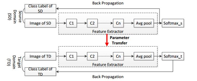
    Citation: Eric Ke Wang, Fan Wang, Ruipei Sun, Xi Liu. A new privacy attack network for remote sensing images classification with small training samples[J]. Mathematical Biosciences and Engineering, 2019, 16(5): 4456-4476. doi: 10.3934/mbe.2019222

    Related Papers:

    [1] Christian Winkel, Simon Neumann, Christina Surulescu, Peter Scheurich . A minimal mathematical model for the initial molecular interactions of death receptor signalling. Mathematical Biosciences and Engineering, 2012, 9(3): 663-683. doi: 10.3934/mbe.2012.9.663
    [2] Hong Yuan, Jing Huang, Jin Li . Protein-ligand binding affinity prediction model based on graph attention network. Mathematical Biosciences and Engineering, 2021, 18(6): 9148-9162. doi: 10.3934/mbe.2021451
    [3] Yuewu Liu, Mengfang Zeng, Shengyong Liu, Chun Li . Dynamics analysis of building block synthesis reactions for virus assembly in vitro. Mathematical Biosciences and Engineering, 2023, 20(2): 4082-4102. doi: 10.3934/mbe.2023191
    [4] Ronald Lai, Trachette L. Jackson . A Mathematical Model of Receptor-Mediated Apoptosis: Dying to Know Why FasL is a Trimer. Mathematical Biosciences and Engineering, 2004, 1(2): 325-338. doi: 10.3934/mbe.2004.1.325
    [5] Feng Rao, Carlos Castillo-Chavez, Yun Kang . Dynamics of a stochastic delayed Harrison-type predation model: Effects of delay and stochastic components. Mathematical Biosciences and Engineering, 2018, 15(6): 1401-1423. doi: 10.3934/mbe.2018064
    [6] Max-Olivier Hongler, Roger Filliger, Olivier Gallay . Local versus nonlocal barycentric interactions in 1D agent dynamics. Mathematical Biosciences and Engineering, 2014, 11(2): 303-315. doi: 10.3934/mbe.2014.11.303
    [7] Yutong Man, Guangming Liu, Kuo Yang, Xuezhong Zhou . SNFM: A semi-supervised NMF algorithm for detecting biological functional modules. Mathematical Biosciences and Engineering, 2019, 16(4): 1933-1948. doi: 10.3934/mbe.2019094
    [8] O. E. Adebayo, S. Urcun, G. Rolin, S. P. A. Bordas, D. Trucu, R. Eftimie . Mathematical investigation of normal and abnormal wound healing dynamics: local and non-local models. Mathematical Biosciences and Engineering, 2023, 20(9): 17446-17498. doi: 10.3934/mbe.2023776
    [9] Zhenzhen Zheng, Ching-Shan Chou, Tau-Mu Yi, Qing Nie . Mathematical analysis of steady-state solutions in compartment and continuum models of cell polarization. Mathematical Biosciences and Engineering, 2011, 8(4): 1135-1168. doi: 10.3934/mbe.2011.8.1135
    [10] Linlu Song, Shangbo Ning, Jinxuan Hou, Yunjie Zhao . Performance of protein-ligand docking with CDK4/6 inhibitors: a case study. Mathematical Biosciences and Engineering, 2021, 18(1): 456-470. doi: 10.3934/mbe.2021025
  • Solving overfitting problems of privacy attacks on small-sample remote sensing data is still a big challenge in practical application. We propose a new privacy attack network, called joint residual network (JRN), for deep learning based privacy objects classification of small-sample remote sensing images in this paper. Unlike the original residual network structure, which add the bottom feature map to top feature map, JRN fuses the bottom feature map with top feature map by matrix joint. It can reduce the possibility that convolution layers extract the noise of training set or consider the inherent attributes of training set as the whole sample attributes. A series benchmark experiments based on GoogleNet model have been enforced and finally, we compare the model process output and the classification accuracy on small-sample data sets. On the UCMLU data set, the GoogleNet-Feat model which is integrated with JRN is 1.66% higher of accuracy than the original GoogleNet model and 1.87% higher than the GoogleNet-R model; on the WHU-RS dataset, GoogleNet-Feat model is 1.04% higher than the GoogleNet model, and is 3.12% higher than the GoogleNet-R model. Compared with the contrast experiments, the classification accuracy of GoogleNet-Feat is the highest when facing the overfitting problems resulting from the small samples.


    Ligands, are biochemical modifiers of macromolecular structure and can impact biological function. These can be co-factors (iron, cobalt, copper, zinc), co-enzymes such as Nicotinamide- and Flavin- Adenine Dinucleotides (NAD, FAD) and full-length molecules with short binding sites [1,2]. Ligands, unlike substrates/co-substrates are either reversibly altered or not at all. The biochemical role of ligands, in vivo, is complex and can influence both, enzyme-mediated substrate catalysis and non-enzymatic association and dissociation interactions. Whilst, the interaction with competitive inhibitors, co-factors or co-enzymes involves definitive and direct modifications to the active site residues, the effect of a ligand can be allosteric and indirect [3,4,5]. The latter involves both long-distance conformational changes and non-covalent interactions (hydrogen, Van der Waals, hydrophobic, electrostatic) [6,7,8,9,10,11]. Empirical data suggests that the binding affinity or the strength-of-association of a macromolecule for its ligand is a critical determinant of function [7,8,9,10,11]. For example, 2, 3-Bisphophoglycerate is a potent modifier of Hemoglobin function and does so by shifting the oxygen-dissociation curve to the right. In its absence Hemoglobin retains high affinity for molecular oxygen (left-shift of the oxygen dissociation curve), an undesirable effect on its role as a transporter [10,11]. Similarly, Ascorbic acid maintains iron in its reduced state in the gastrointestinal tract and as part of the active site of non-haem iron (Ⅱ)- and 2-oxoglutarate-dependent dioxygenases [12,13]. Deficiency of Ascorbic acid is implicated in tardy iron absorption in the ileum as well as a range of collagen disorders such as scurvy (Prolyl- and Lysyl-hydroxylases) [14,15]. Conversely, proteins which are modified such as those that may originate from missense or amino acid substitutions and are secondary to genomic variants such as single nucleotide polymorphisms (SNPs) and insertions-deletions (indels), will also result in several clinical outcomes [16,17]. Here, too, enzyme catalysis is directly affected if these are present at the active site or is impacted indirectly (folding, stability, complex formation) when present elsewhere [16,17,18].

    There is a large volume of literature which describes macromolecules in terms of either residues (amino acids, nucleotides) interacting or an all atom-based interaction matrix. The proponent of the 2D approach is the Gaussian network model (GNM), while the Anisotropic network model (ANM) is representative of the 3D approach [19,20,21,22]. The fundamental premise of both these approaches is the elastic network model (ENM) [19]. Here, an atom or residue is modeled as an elastic mass and the interaction between a pair of atoms/residues is dependent on the selection of a pre-determined cut-off distance [22]. The force constant, although, not a parameter by definition, has also been studied and shows good correlation with B-factor data [23]. A major application of these studies is normal mode analysis (NMA), which has been used to glean valuable insights into the structural dynamics of the investigated macromolecule and into B-factor distribution [23,24]. Despite this success, there are significant limitations of this approach, including inadequate descriptors for the type of interactions computed by the Hessian matrix and data points that are dependent on a preselected cut-off distance (5–10 Ang, GNM; 10–15 Ang, ANM) [20,22,25]. Parameter-free versions of the ENM (pfENM), GNM (pfGNM) and ANM (pfANM), to resolve the latter, have been described and compared to establish B-factor distribution (isotropic, anisotropic) [25]. Additionally, many of these studies have focused on inferring biophysical characteristics such as cross-correlational fluctuations and mean square displacements. From a functional standpoint, however, it is not clear whether these data can be utilized to derive/study parameters such as the Michaelis-Menten constant (Km) or the association/dissociation (Ka/Kd). Since, these depend on the presence of an organic or inorganic modifier, i.e., ligand/substrate/co-factor/co-substrate, in addition to the modeled macromolecule, its exclusion is another major lacuna of these studies.

    Despite the availability of clinical, empirical, analytical and computational data, a mathematically rigorous explanation for the heterogeneity in biochemical function, for a ligand-macromolecular complex, is missing. The work presented models a ligand and macromolecule as a homo- or hetero-dimer and subsumes a finite and equal number of atoms/residues per monomer. The pairwise interactions of the resulting square matrix will be chosen randomly from a standard uniform distribution. The resulting eigenvalues will be analyzed and modeled in accordance with known literature on biochemical reactions to generate biologically viable and usable dissociation constants. The theoretical results will be complemented by numerical studies where applicable. Additionally, and through various theorems, lemmas and corollaries, a schema to partition ligands into high- and low-affinity variants will also be discussed. The suitability of the transition-state dissociation constants as a model for ligand-macromolecular interactions will be inferentially assessed by analyzing the clinical outcomes of amino acid substitutions of selected enzyme homodimers. The relevance of the model to biochemical function will be discussed by examining the ligand-macromolecular complex for known ligands of non-haem iron (Ⅱ)- and 2-oxoglutarate-dependent dioxygenases (Fe2OG) and the major histocompatibility complex (Ⅰ) (MHC1).

    The general outline of the manuscript includes an initial section where the system to be modeled, rationale for this study, and formal definitions are introduced (Section 2). The model is analyzed, formulated and presented as theorems, lemmas and corollaries (Section 3). This section also includes a numerical study to demonstrate and validate the theoretical assertions made. The biological relevance of these findings are discussed with an analysis of clinical outcomes of enzyme sequence variants and case studies of enzyme- and non-enzymatic complex formation (Section 4). A brief conclusion that summarizes the presented study, limitations and future directions is included at the end of the manuscript (Section 5). Details of all proofs are included after the conclusions (Section 6).

    Consider the generic interaction between macromolecule (c) and ligand (μ),

    cμrfrbc+μRXN(1)

    We can represent this interaction/reaction, at a steady state, with the rate equations [26],

    Rd(cμ)=rf.[cμ]Lcμ0 (1)
    Ra(cμ)=rb.[c]Lc0[μ]Lμ0 (2)

    At steady state,

    Rd(cμ)=Ra(cμ) (3)
    rfrb=[c]Lc0.[μ]Lμ0[cμ]Lcμ0 (4)
    rfrb=Kd(cμ) (5)

    Here,

    c:=Macromolecule
    μ:=Ligand
    [.]:=Molarconcentrationofreactantinstandardform(M)
    Ra(cμ):=Rateofassociationofcomplex(Ms1)
    Rd(cμ):=Rateofdissociationofcomplex(Ms1)
    rf:=Rateconstantsofforwardreaction(s1)
    rb:=Rateconstantsofreversereaction(M1s1)
    L:=Stoichiometryofreactant(s)
    Kd(cμ):=Dissociationconstantforligandmacromolecularcomplex(M)

    It is clear that a ligand-macromolecular complex may exist in one of three distinct states. These include: a) perfect association, b) perfect dissociation and c) an intermediate- or transition-state; and can be represented in terms of the dissociation constant,

    Case (1)     Perfectassociation      Def. (1)

    1rb;rf0 (6, 7)
    Kd(cμ)0 (8)

    Case (2)    Perfectdisassociation    Def. (2)

    rf>>>rb (9)
    Kd(cμ)1 (10)

    Case (3)    Transientstatedisassociationconstant    Def. (3)

    rfrb (11)
    Kd(cμ)R(0,1) (12)

    Consider an atom/residue-based representation (amino acids/nucleotides) of a generic set of monomeric macromolecules, {\boldsymbol{\mathcal{C}}} = \{protein, DNA, RNA\} , with z = \mathrm{1, 2}, \dots ., Z components each with i -indexed ( i = \mathrm{1, 2}, \dots ., I ) c-atoms/residues,

    \begin{array}{cc}{{\bf c}\equiv {{{\mathcal{C}}}}_{z}\in {\boldsymbol{\mathcal{C}}}|{\bf c} = \left[{c}_{1}{c}_{2}\dots .{c}_{i = I}\right]}^{T}, I\in \mathbb{N}& \end{array} (13)

    The analogous model of a monomer ligand, {\boldsymbol{\mathcal{L}}} = \{small\;molecule, peptide, oligonucleotide\} , with j -indexed (j = \mathrm{1, 2}, \dots , J) \mu -atoms/residues is,

    \boldsymbol{\mu }\in {\boldsymbol{\mathcal{L}}}|{\bf{ \pmb{\mathsf{ μ}} }} = \left[{\mu }_{1}{\mu }_{2}\dots .{\mu }_{j = J}\right], J\in \mathbb{N} (14)

    It is also assumed that the ligand-macromolecular complex is a homo- or hetero-dimer with an equal number of atoms/residues \left(I = J\right) per monomer. The interaction matrix is,

    \begin{array}{rr}\left\langle{\boldsymbol{c}|\boldsymbol{\mu }}\right\rangle = {\left[{c}_{1}{c}_{2}..{c}_{i = I}\right]}^{T}\times \left[{\mu }_{1}{\mu }_{2}..{\mu }_{j = J}\right] = {{\boldsymbol{\mathcal{C}}}}_{\boldsymbol{z}\boldsymbol{\mu }} = \left({{c}_{i}\mu }_{j}\right)\subset {\mathbb{R}}^{I\times J}& \end{array} (15)

    The numerical values of this matrix are chosen randomly from the standard uniform distribution,

    \begin{array}{rr}{{\boldsymbol{\mathcal{C}}}}_{z\mu } = \left({{c}_{i}\mu }_{j}\right)\in {\mathcal{U}}_{\left[\mathrm{0, 1}\right]}& \end{array} (16)

    The rationale for this choice is that each pairwise interaction is subsumed to be a function of an arbitrary number of non-bonded interactions (long- and short-range) and is therefore, unique. Clearly, this implies the existence of \left\{I, J\right\} -linear independent vectors,

    \begin{array}{cc}rank\left({{\boldsymbol{\mathcal{C}}}}_{z\mu }\right) = \left\{I, J\right\}& \end{array} (17)

    Since {{\boldsymbol{\mathcal{C}}}}_{\boldsymbol{z}\boldsymbol{\mu }} is diagonalizable there exists a diagonal matrix, \mathit{\boldsymbol{\mathcal{K}}{\boldsymbol{\mathcal{C}}}}_{z\mu } ,

    \mathit{\boldsymbol{\mathcal{K}}{\boldsymbol{\mathcal{C}}}}_{z\mu } = {\boldsymbol{X}}^{-1}{{\boldsymbol{\mathcal{C}}}}_{z\mu }\boldsymbol{X} (18)
    {z}_{i = j} = z\in diag\left(\mathit{\boldsymbol{\mathcal{K}}{\boldsymbol{\mathcal{C}}}}_{z\mu }\right)\subset \mathbb{C} (19)

    {{\boldsymbol{\mathcal{C}}}}_{\boldsymbol{z}\boldsymbol{\mu }} , is non-symmetric the computed eigenvalues of the modeled ligand-macromolecular interaction matrix can have positive and negative real parts,

    \left\{{\alpha }_{ij} = Re\left(z\right)\in \boldsymbol{K}\boldsymbol{d}\left({{\boldsymbol{\mathcal{C}}}}_{\boldsymbol{z}\boldsymbol{\mu }}\right)\subset \mathbb{R}|i = j, z\in \mathbb{C}\right\} (20)
    \left\{{\alpha }_{ij} = Re\left(z\right)\in \boldsymbol{K}\boldsymbol{d}\left({{\boldsymbol{\mathcal{C}}}}_{\boldsymbol{z}\boldsymbol{\mu }}\right)\subset \mathbb{R}|i = j, z\in \mathbb{C}\right\} (20.1)

    A further subdivision can be made in accordance with established literature,

    \left\{{\alpha }_{ij} = Re\left(z\right)\in \boldsymbol{K}\boldsymbol{d}\left({{\boldsymbol{\mathcal{C}}}}_{\boldsymbol{z}\boldsymbol{\mu }}\right)\subset \mathbb{R}|i = j, z\in \mathbb{C}\right\} {\omega }_{\infty } = Kd\left(c\mu \right)\ge 1 (21)
    Perfect\;association\equiv Reverse \;\; {\omega }_{0} = Kd\left(c\mu \right) = 0 (22)

    This selection generates the set,

    \omega = {\alpha }_{ij}\in \boldsymbol{K}\boldsymbol{d}\left({{\boldsymbol{\mathcal{C}}}}_{\boldsymbol{z}\boldsymbol{\mu }}\right)\subset \mathbb{R}\cap \left(\mathrm{0, 1}\right) (23)
    \omega \in \boldsymbol{K}\boldsymbol{d}\left(\boldsymbol{c}\boldsymbol{\mu }\right)\;\;\;\;\;\;\;\;\;\;\;\;\;\;\;\;\;\;\;\;\;\;\;\;\;\;\;\;\;Def.\; {\mathit{(4)}}
    \#\boldsymbol{K}\boldsymbol{d}\left(\boldsymbol{c}\boldsymbol{\mu }\right) = A (23.1)

    We can combine these to get a preliminary definition of the transition-state disassociation constants. These are the strictly positive real part of all complex eigenvalues that characterize a ligand-macromolecular complex with an equal number of atoms/residues per monomer and belong to the open interval (0, 1),

    \left\{\omega = \mathcal{R}\mathrm{e}\left(\mathrm{z}\right)\in \boldsymbol{K}\boldsymbol{d}\left(\boldsymbol{c}\boldsymbol{\mu }\right)\subset \boldsymbol{K}\boldsymbol{d}\left({{\boldsymbol{\mathcal{C}}}}_{\boldsymbol{z}\boldsymbol{\mu }}\right)\subset \mathbb{R}\cap \left(\mathrm{0, 1}\right)|z\in \mathbb{C}\right\} (Def. \; {\mathit{(5a)}})

    Whilst, the states of perfect association and dissociation are key determinants of whether a reaction will occur or not, the transition-state dissociation constants may offer insights into the origins of threshold values, feedback mechanisms and other regulatory checkpoints. However, in order to ascribe biological relevance to these findings we must establish various bounds which can then be utilized to assess and thence assay the function of a ligand-macromolecular complex.

    Theorem 1 (T1): The linear map between the transition-state dissociation constants and the eigenvalues that characterize the interactions of the homo- or hetero-dimer form of the modeled ligand-macromolecular complex is the injection,

    g:\omega \in \boldsymbol{K}\boldsymbol{d}\left(\boldsymbol{c}\boldsymbol{\mu }\right)\mapsto \boldsymbol{K}\boldsymbol{d}\left({{\boldsymbol{\mathcal{C}}}}_{\boldsymbol{z}\boldsymbol{\mu }}\right) (24)

    Theorem 2 (T2): The transition-state dissociation constants that characterize the interactions of the homo- or hetero-dimer form of the modeled ligand-macromolecular complex is a monotonic and non-increasing sequence,

    \begin{array}{cc}{\left\{{\omega }_{a}\right\}}_{a\le a+1}|& \omega \in \boldsymbol{K}\boldsymbol{d}\left(\boldsymbol{c}\boldsymbol{\mu }\right)\end{array} (25)

    Theorem 3 (T3): The transition-state dissociation constants that characterize the interactions of the homo- or hetero-dimer form of the modeled ligand-macromolecule complex are monotonic, bounded and therefore, convergent,

    \begin{array}{cc}\underset{a\to \infty }{\mathrm{lim}}{\left\{{\omega }_{a}\right\}}_{a\le a+1} = \left\{\mathrm{0, 1}\right\}|& \omega \in \boldsymbol{K}\boldsymbol{d}\left(\boldsymbol{c}\boldsymbol{\mu }\right)\end{array} (26)

    Corollary 1 (C1): The transition-state dissociation constants that characterize the interactions of the homo- or hetero-dimer form of the modeled ligand-macromolecule complex is a sequence with defined greatest-lower and least-upper -bounds,

    inf{\left\{{\omega }_{a}\right\}}_{a\le a+1} < {\left\{{\omega }_{a}\right\}}_{a\le a+1} < sup{\left\{{\omega }_{a}\right\}}_{a\le a+1} (27)

    Corollary 2 (C2; without proof): The cardinality of the set of transition-state dissociation constants that characterize the interactions of the homo- or hetero-dimer form of the modeled ligand-macromolecule complex is finite,

    \begin{array}{c}\#\boldsymbol{K}\boldsymbol{d}\left(\boldsymbol{c}\boldsymbol{\mu }\right) = A < \#\boldsymbol{K}\boldsymbol{d}\left({{\boldsymbol{\mathcal{C}}}}_{\boldsymbol{z}\boldsymbol{\mu }}\right) = \left\{I, J\right\}\end{array} (28)

    Using T1–T3 and C1, C2 we can refine our definition of the transition-state dissociation constants for the modeled ligand-macromolecular complex,

    \begin{array}{cc}{\left\{{\omega }_{a}\right\}}_{a\le a+1}|& \omega \in \boldsymbol{K}\boldsymbol{d}\left(\boldsymbol{c}\boldsymbol{\mu }\right)\end{array};a = \mathrm{1, 2}\dots A (Def. \; {\mathit{(5b)}})

    where,

    \omega = \mathcal{R}\mathrm{e}\left(\mathrm{z}\right)\in \boldsymbol{K}\boldsymbol{d}\left({{\boldsymbol{\mathcal{C}}}}_{\boldsymbol{z}\boldsymbol{\mu }}\right)\subset \mathbb{R}\cap \left(\mathrm{0, 1}\right)|z\in \mathbb{C}

    It is clear from the above results that the eigenvalue-based transition-state dissociation constants are continuous and can potentially model the multiplicity of intermediate- or transient-states that a ligand-macromolecular complex may adopt. It should therefore, be possible to partition the transition-state dissociation constants into functionally distinct subsets and will be characteristic for a specific ligand-macromolecular complex.

    Theorem 4 (T4): The transition-state dissociation constants that characterize the interactions of the homo- or hetero-dimer form of the modeled ligand-macromolecule complex is a proper subset of the complete set of the real part of all complex eigenvalues that comprise the interaction matrix,

    \boldsymbol{K}\boldsymbol{d}\left(\boldsymbol{c}\boldsymbol{\mu }\right)\subset \boldsymbol{K}\boldsymbol{d}\left({{\boldsymbol{\mathcal{C}}}}_{\boldsymbol{z}\boldsymbol{\mu }}\right) (29)

    Corollary 3 (C3): The distribution of the transition-state dissociation constants that characterize the interactions of the homo- or hetero-dimer form of the modeled ligand-macromolecule complex will result in a schema by which we can annotate the ligand as a high \left({\mu }_{high}\right) - or low \left({\mu }_{low}\right) -affinity variant,

    \mu = \left\{{\mu }_{high}, {\mu }_{low}\right\} (30)

    Biologically relevant macromolecular complexes are characterized by heterogeneity and high-order \left(Z\ge 2\right) . This multimer-form of a macromolecule is formed around a primary molecule and its interactions. These may be protein-protein, DNA/RNA-protein or DNA-RNA-protein.

    The multimer-form of ligand-macromolecular complex is easily modeled using the mathematical framework defined earlier. Here, the ligand-macromolecular complex is considered as a set of interacting monomers and the binding to a ligand occurs via a single unique monomer,

    \left\{{{{\mathcal{C}}}}_{z}\in {\boldsymbol{\mathcal{C}}}|{{{\mathcal{C}}}}_{1} = {{{\mathcal{C}}}}_{2}\dots = {{{\mathcal{C}}}}_{z = Z}|Z\ge 2\right\} (Def. \; {\mathit{(6a)}})

    where,

    {{{\mathcal{C}}}}_{z}\equiv {{{\mathcal{C}}}}_{z\mu }\equiv \mu {{{\mathcal{C}}}}_{z} (Def. \; {\mathit{(6b)}})

    Here,

    \mu : = Ligand
    {{{\mathcal{C}}}}_{z}: = Unique\;monomer\;of\;a\;macromolecule\;that\;associates\;with\;a\;ligand
    \mu {{{\mathcal{C}}}}_{z}: = Ligand-macromolecular\;complex

    On the basis of these definitions we can re-index the remaining monomers, i.e., after excluding the unique monomer that binds to the ligand,

    \left\{{{{\mathcal{C}}}}_{y}\in \widetilde {{\boldsymbol{\mathcal{C}}}} = {\boldsymbol{\mathcal{C}}}\backslash \left\{{{{\mathcal{C}}}}_{z}\right\}|y = \mathrm{1, 2}\dots Y;Y = Z-1\right\} (Def. \; {\mathit{(7)}})

    We now derive an expression for the multimer (higher-order)-form of a ligand-macromolecular complex.

    Theorem 5 (T5): The multimer-form of a ligand-macromolecular complex comprising identical monomer units and with an arbitrary unit associating with a ligand is,

    \begin{array}{rr}{\prod }_{y = 1}^{y = Y}{{{\mathcal{C}}}}_{z}.{\mathcal{C}}_{y} = {\mathcal{C}}_{z}.{\mathcal{C}}_{Y}^{y}|y = \mathrm{1, 2}\dots Y;Y = Z-1;Z\ge 2;z = \mathrm{1, 2}\dots Z& \end{array} (31)

    Rewriting, this result in terms of the definition of the multimer form of a ligand-macromolecular complex,

    \begin{array}{cc}{\mathcal{C}}_{z}.{\mathcal{C}}^{Y}\equiv \mu {\mathcal{C}}_{z}.{\mathcal{C}}^{Y}& \end{array} (Def. \; {\mathit{(8)}})

    Theorem 6 (T6): The linear map between the transition-state dissociation constants that characterize the interactions of the monomer- and multimer-forms of a ligand-macromolecular complex is a bijection,

    \begin{array}{cc}{h}^{-1}\circ h:\omega \in \boldsymbol{K}\boldsymbol{d}\left(\boldsymbol{c}\boldsymbol{\mu }\right)\leftrightarrow u\in \boldsymbol{K}\boldsymbol{d}\left(\mu \boldsymbol{\mathcal{C}}_{z}\right)& \end{array} (32)

    Theorem 7 (T7): The linear map between the transition-state dissociation constants and the eigenvalues that characterize the multimer-form of a ligand-macromolecular complex is a composition and an injection,

    \begin{array}{cc}g\circ {h}^{-1}\circ h:u\in \boldsymbol{K}\boldsymbol{d}\left(\mu \boldsymbol{\mathcal{C}}_{z}.{\mathcal{C}}^{Y}\right)\mapsto \boldsymbol{K}\boldsymbol{d}\left(\boldsymbol{\mathcal{C}}_{\boldsymbol{z}\boldsymbol{\mu }}\right)& \end{array} (33)

    The aforementioned theoretical results establish the mathematical rigor behind the definition and development of the transition-state dissociation constants as a model for ligand-macromolecular interactions (T1–T7, C1–C3). These assertions are complemented and numerically validated in R-4.1.2. Here, the R-packages, "ConvergenceConcepts" and "pracma" are utilized to investigate and analyze the stochastic convergence of the eigenvalues generated by the interaction matrix of a ligand-macromolecular complex (Supplementary Text 1) [27]. The R-scripts to establish convergence along with data processing are developed in-house (Supplementary Text 2). The stepwise algorithm to compute and numerically validate the transition-state dissociation constants is presented (Figure 1).

    Figure 1.  Numerical studies of ligand-macromolecular interactions as eigenvalue-based transition-state dissociation constants.

    Step 1: A ligand and macromolecule with an equal number of atoms/residues ( n = 25 ) is chosen. Whilst, the complex can be modeled as a perfect homodimer, imperfect forms such as alternatively spliced isoenzymes are prevalent and commonly observed. Alternatively, the ligand can be modeled as a different macromolecule altogether.

    Step 2: Populate the square interaction matrix with values randomly chosen from a uniform distribution, {\mathcal{U}}_{\left[\mathrm{0, 1}\right]} . These will represent one of three potential states for each interacting pair of atoms/residues of the modeled ligand-macromolecular complex (association, complete disassembly, transition-state).

    Step 3: Compute the complex eigenvalues of this matrix and extract the real part of each.

    Step 4: Form a sequence of the subset comprising those values that are strictly positive and belong to the open interval \left(\mathrm{0, 1}\right) .

    Step 5: Establish the stochastic convergence in distribution and/or probability of the terms of this sequence to the expected upper (tsup)- and lower (tinf)-bounds, i.e., 0 and 1.

    Step 5.1: Construct a sequence of random numbers, X, whose elements are uniquely mapped to the eigenvalue-based transition-state dissociation constants and represent intermediate- or transition-states of the modeled ligand-macromolecular complex,

    \left\{{X}_{a}\in \boldsymbol{X}\cap \boldsymbol{K}\boldsymbol{d}\left(\boldsymbol{c}\boldsymbol{\mu }\right)\subset \mathbb{R}\cap \left(\mathrm{0, 1}\right)|a = \mathrm{1, 2}\dots A\right\} (Def. \; {\mathit{(9)}})

    Here,

    A = \#\left(\boldsymbol{X}\cap \boldsymbol{K}\boldsymbol{d}\left(\boldsymbol{c}\boldsymbol{\mu }\right)\right) (34)

    Step 5.2: Establish convergence of this set of random numbers. Here, weak convergence will suffice (distribution, probability),

    \underset{a\to \infty }{\mathrm{lim}}\left({X}_{a}\right)\to \left\{tinf, tsup\right\} = \left\{\mathrm{0, 1}\right\} (35)

    The parameters to accomplish this numerically are,

    \begin{array}{r}nmax: = Number\;of\;values\;to\;analyse\\ M: = Number\;of\;paths\\ \varepsilon : = Threshold\;value\\ tinf: = Lower\;limit\;of\;interval\;to\;establish\;convergence\\ tsup: = Upper\;limit\;of\;interval\;to\;establish\;convergence\end{array}

    The values of these parameters for the numerically studied example are,

    nmax = A = 11 (35.1)
    M = 500 (35.2)
    \varepsilon = 0.01 (35.3)
    tinf = 0 (35.4)
    tsup = 1 (35.5)

    The eigenvalue-based model of transition-state dissociation constants of a ligand-macromolecular complex asserts that there are several intermediate- or transition-states of a complex and that each of these has the potential to modify the biochemical process that the complex participates in.

    Ligand-macromolecular complexes, in vivo, possess a finite and in most cases, an incomparable number of atoms/residues. The theoretical results establish definition(s), bounds and metrics to assess biochemical function for both, monomer (T1–T4, C1–C3)- and multimer (T5–T7)-forms. The numerical data suggests that the set of transition-state dissociation constants can be finite, converge and retain statistical relevance (Figure 1).

    Proposition (P): The transition-state dissociation constants for the monomer ( z = Z = 1 )- and multimer ( Z\ge 2 )-forms of a ligand-macromolecular complex with a finite number of atoms/residues of each \left(I, J\right) per monomer,

    \left\{u\in \boldsymbol{K}\boldsymbol{d}\left(\boldsymbol{\mu }\boldsymbol{\mathcal{C}}_{\boldsymbol{z}}.\boldsymbol{\mathcal{C}}^{\boldsymbol{Y}}\right)|{\mathcal{C}}_{z}\in \boldsymbol{\mathcal{C}}, \mu \in {\boldsymbol{\mathcal{L}}};z = \mathrm{1, 2}\dots Z;A = \left\{I, J\right\}\right\} (Def. \; {\mathit{(10)}})

    is the finite set,

    \boldsymbol{K}\boldsymbol{d}\left(\boldsymbol{\mu }\boldsymbol{\mathcal{C}}_{\boldsymbol{z}}.\boldsymbol{\mathcal{C}}^{\boldsymbol{Y}}\right)\subset \boldsymbol{K}\boldsymbol{d}\left(\boldsymbol{\mathcal{C}}_{\boldsymbol{z}\boldsymbol{\mu }}\right)

    Here,

    I = \#{\mathcal{C}}_{z}|{\mathcal{C}}_{z}\in \boldsymbol{\mathcal{C}} (36)
    J = \#\mu |\mu \in {\boldsymbol{\mathcal{L}}} (37)

    where,

    \boldsymbol{K}\boldsymbol{d}\left(.\right): = Set\;of\;constrained\;eigenvalue-based\;transition-state\;dissociation\;constants
    I: = Finite\;number\;of\;atoms\;or\;residues\;of\;macromolecule
    J: = Finite\;number\;of\;atoms\;or\;residues\;of\;ligand
    {\mathcal{C}}_{\mu z}.{\mathcal{C}}^{Y}: = Multimer\;form\;of\;ligand-macromolecular\;complex

    Enzyme-mediated catalysis, or lack thereof, results in metabolic enzyme disorders and may be inherited (inborn errors of metabolism) or acquired [28]. In order to assess the biomedical relevance of modeling ligand-macromolecule interactions as transition-state dissociation constants, the clinical outcomes of amino acid substitutions of selected enzyme homo- or hetero-dimers are examined (Table 1). These outcomes, i.e., benign, likely benign, pathologic, likely pathologic, conflicting, uncertain significance, are defined in accordance with the prevalent nomenclature of the ClinVar database [16]. Here, the data annotated as "uncertain significance" are those sequence variants with a high likelihood ( \approx 90–95\% ) of being "benign" or "pathogenic" [17]. This means they are likely to classified as "true positive", and if ignored will result in a "false negative". On the other hand, an outcome designated as with a "conflicting interpretation" is likely to be due to unresolved contradictory findings in the presence or absence of confounding factors. If we assume perfect contradiction, i.e., 50%, and couple this with the previous result, we get a \approx 70–73\% possibility that the variant of interest is a "true positive". This means, that here too, if missed a "false negative" will result. The metric of choice is the Recall (R) percentage,

    R = \frac{TP}{TP+FN}\times 100 (38)
    R: = Recall
    \begin{array}{l} TP: = Known\;positives(benign, likelybenign,\\ pathogenic, likely\;pathogenic) \end{array} (Def. \; {\mathit{(12)}})
    \begin{array}{l} FN: = Likely\;positives(conflicting\\ \;data, uncertain\;significance) \end{array} (Def. \; {\mathit{(13)}})
    Table 1.  Analysis of clinical outcomes of amino acid substitutions of selected enzyme homo- and hetero-dimer forms present in ClinVar.
    Enzyme EC CV SNP M Co US B LB P LP FN TP R (%)
    1 Glucokinase 2.7.1.2 778 619 370 49 157 4 4 65 113 206 186 47.45
    2 Pyruvate kinase 2.7.1.40 1239 629 209 14 135 7 7 30 20 149 64 30.05
    3 Cathepsin A 3.4.16.x 1776 1270 501 20 382 26 23 26 34 402 109 21.33
    4 Pyruvate dehydrogenase 1.2.4.1 2317 1591 584 25 391 35 46 62 43 416 186 30.9
    5 Phosphofructokinase 1 2.7.1.11 165 32 10 2 4 2 1 1 1 6 5 45.45
    6 Phosphofructokinase 2 2.7.1.105 206 76 23 1 17 1 1 2 1 18 5 21.74
    7 Cystathione beta-synthase 4.2.1.22 930 744 255 21 172 3 4 46 32 193 85 30.58
    8 DNA topoisomerase Ⅱ 5.6.2.2 466 319 152 0 122 11 14 3 1 122 29 19.21
    9 Guanylate cyclase 1 4.6.1.2 1572 1117 576 29 417 11 10 34 59 446 114 20.36
    10 Phenylalanine hydroxylase 1.14.16.1 1314 1102 631 5 182 0 3 161 254 187 418 69.09
    Note: EC: Enzyme commission number; CV: Number of clinical variants; SNP: Single nucleotide polymorphisms; M: Missense mutations; Co: Conflicting data; US: Uncertain significance; B: Benign; LB: Likely; P: Pathogenic; LP: Likely pathogenic; FN: False negative (Co + US); TP: True positive (B + LB + P + LP); R: Recall ( \frac{TP}{TP+FN}\times 100 ).

     | Show Table
    DownLoad: CSV

    It is clear from these data that amino acid substitutions (nature, type), either alone or in combination, comprise distinct transition-states and are significant contributors to the biochemical function of each enzyme dimer ( Recall\approx 19–70\% ). Since each of these states will result in a distinct Kd , it is easily inferred that the transition-state dissociation constants, for a complex, may be more representative of biochemical function (T1–T4, C1–C3).

    The discussion, vide supra, presents and highlights the biomedical relevance of modeling ligand-macromolecular interactions as transition-state dissociation constants. The results for monomer- and multimer-forms of ligand-macromolecular complexes are mathematically rigorous and have been validated, in silico. The results are now examined in context of biochemical function (enzyme, non-enzyme) for selected cases.

    Case 1: Oxygen sensitive variants of non-haem iron (II)- and 2-oxoglutarate-dependent dioxygenases

    The non-haem iron (Ⅱ)- and 2-oxoglutarate-dependent dioxygenases \left(EC1.14.x.y\right) , comprise a large superfamily of enzymes, are present in all kingdoms of life and is chemically diverse (variable reaction chemistry, multiple substrates) [12,13,29]. Clinically relevant members include Phytanoyl-CoA dioxygenase (PHYT), Lysine Hydroxylases, and the Proline 4-Hydroxylases (P4H) amongst several others [12,13,14,15,29]. These enzymes have important roles in Phytanic acid metabolism and collagen maturation, with sub-optimal activities contributing to diseases such as Refsum and the Ehlers-Danlos (ED)-syndrome [14,15,30]. Here, too, the outcomes (clinical, non-clinical) associated with substitution mutations for PHYT suggest that modeling ligand-macromolecular interactions as transition-state dissociation constants may be a better index of biochemical function (T1T4, C1C3, P) [31].

    P4Hs, are classified as being either hypoxia-sensitive \left(H-P4H\equiv HP4H;EC\mathrm{1.14.11.29}\right) or collagen transforming \left(C-P4H\equiv CP4H;EC\mathrm{1.14.11.2}\right) [28]. These reactions may be written,

    \begin{array}{rr}HP4H-HIF+{O}_{2}+2OG+Proline\begin{array}{c}\stackrel{{r}_{f}}{\to }\\ \underset{{r}_{b}}{\leftarrow }\end{array}Hydroxyproline+SA+{CO}_{2}& RXN\left(2\right)\\ CP4H+{O}_{2}+2OG+Proline\begin{array}{c}\stackrel{{r}_{f}}{\to }\\ \underset{{r}_{b}}{\leftarrow }\end{array}Hydroxyproline+SA+{CO}_{2}& RXN\left(3\right)\end{array}
    \begin{array}{rrr}{r}_{f}, {r}_{b}& : = & Rate\;constants\;for\;forward\;and\;backward\;reactions\;at\;steady\;state\\ HP4H& : = & Hypoxia\;inducible\;factor-dependent\;Proline\;4-Hydroxylase\\ HIF\equiv {\mu }_{high}& : = & Hypoxia-inducible\;factor(high-affinity\;modifier)\\ 2OG& : = & 2-oxoglutarate\\ SA& : = & Succinic\;acid\\ C{O}_{2}& : = & Carbon\;dioxide\end{array}

    The amino acid identity between HP4H and CP4H notwithstanding, there are significant differences between the molecular biology that they exhibit. This implies that despite the similarity of co-factor \left(iron\left(II\right)\right) , substrate \left(L-Proline\right) and co-substrate \left(2-oxoglutarate\right) , the binding affinities for molecular dioxygen vary considerably [7,32],

    {Km}_{HP4H} = 0.1-0.76\;mM (39)
    {Km}_{CP4H} = 0.03-1.5\;mM (40)

    The turnover numbers for the cognate substrate, too, differ significantly [7],

    {Kcat}_{HP4H} = 0.015-0.733{s}^{-1} (41)
    {Kcat}_{CP4H} = 0.0188-0.02{s}^{-1} (42)

    Clearly, a plausible explanation for these disparate empirical observations is the binding of the hypoxia-inducible factors (HIF) to P4H. The hypoxia-inducible factors (HIFs), are a family (n = 3) of transcription factors which sense hypoxia and trigger the upregulation of hypoxia-dependent genes [32,33,34]. Here, although hypoxia-inducible factor, is a full length protein, the actual binding site is the C-terminal end of HP4H [7,35].

    Kd\approx 0.000016-0.023\;mM (43)

    Some of these observations may be inferred from the partitioning of the transition-state dissociation constants into distinct subsets (Table 2):

    Table 2.  Ligand-macromolecular biochemistry as a function of its transition-state dissociation constants.
    Case 1 Case 2
    Ligand \left(\boldsymbol{\mu }\in {\boldsymbol{\mathcal{L}}}\right) Hypoxia-inducible factor Peptide
    Macromolecule \left(\boldsymbol{c}\equiv {\boldsymbol{\mathcal{C}}}_{\boldsymbol{z}}\in \boldsymbol{\mathcal{C}}\right) HP4H, CP4H M1\beta
    Primary complex \left\langle {} \right.\boldsymbol{c}|\boldsymbol{\mu }\left. {} \right\rangle
    High-affinity variant :=\boldsymbol{K}\boldsymbol{d}\left({\boldsymbol{\mu }}_{\boldsymbol{h}\boldsymbol{i}\boldsymbol{g}\boldsymbol{h}}{\boldsymbol{\mathcal{C}}}_{\boldsymbol{z}}\right)
    Low-affinity variant :=\boldsymbol{K}\boldsymbol{d}\left({\boldsymbol{\mu }}_{\boldsymbol{h}\boldsymbol{i}\boldsymbol{g}\boldsymbol{h}}{\boldsymbol{\mathcal{C}}}_{\boldsymbol{z}}\right)
    \left\langle{\boldsymbol{H}\boldsymbol{P}{\bf{4}}\boldsymbol{H}|\boldsymbol{\mu }}\right\rangle , \left\langle{\boldsymbol{C}\boldsymbol{P}{\bf{4}}\boldsymbol{H}|\boldsymbol{\mu }}\right\rangle
    \boldsymbol{K}\boldsymbol{d}\left(\boldsymbol{H}\boldsymbol{P}{\bf{4}}\boldsymbol{H}|{\boldsymbol{\mu }}_{\boldsymbol{h}\boldsymbol{i}\boldsymbol{g}\boldsymbol{h}}\right)=\boldsymbol{K}\boldsymbol{d}\left({\boldsymbol{\mu }}_{\boldsymbol{h}\boldsymbol{i}\boldsymbol{g}\boldsymbol{h}}\boldsymbol{H}\boldsymbol{P}{\bf{4}}\boldsymbol{H}\right)
    \boldsymbol{K}\boldsymbol{d}\left(\boldsymbol{C}\boldsymbol{P}{\bf{4}}\boldsymbol{H}|{\boldsymbol{\mu }}_{\boldsymbol{l}\boldsymbol{o}\boldsymbol{w}}\right)=\boldsymbol{K}\boldsymbol{d}\left({\boldsymbol{\mu }}_{\boldsymbol{l}\boldsymbol{o}\boldsymbol{w}}\boldsymbol{C}\boldsymbol{P}{\bf{4}}\boldsymbol{H}\right)
    \left\langle{\boldsymbol{M}{\bf{1}}\boldsymbol{\beta }|\boldsymbol{\mu }}\right\rangle
    \boldsymbol{K}\boldsymbol{d}\left(\boldsymbol{M}{\bf{1}}\boldsymbol{\beta }|{\boldsymbol{\mu }}_{\boldsymbol{h}\boldsymbol{i}\boldsymbol{g}\boldsymbol{h}}\right)=\boldsymbol{K}\boldsymbol{d}\left({\boldsymbol{\mu }}_{\boldsymbol{h}\boldsymbol{i}\boldsymbol{g}\boldsymbol{h}}\boldsymbol{M}{\bf{1}}\boldsymbol{\beta }\right)
    \boldsymbol{K}\boldsymbol{d}\left(\boldsymbol{M}{\bf{1}}\boldsymbol{\beta }|{\boldsymbol{\mu }}_{\boldsymbol{l}\boldsymbol{o}\boldsymbol{w}}\right)=\boldsymbol{K}\boldsymbol{d}\left({\boldsymbol{\mu }}_{\boldsymbol{l}\boldsymbol{o}\boldsymbol{w}}\boldsymbol{M}{\bf{1}}\boldsymbol{\beta }\right)
    Higher-order complex \left\langle {} \right.\boldsymbol{c}|\boldsymbol{\mu }\left. {} \right\rangle .{{\mathcal{C}}}^{y}
    High-affinity variant :=\boldsymbol{K}\boldsymbol{d}\left({\boldsymbol{\mu }}_{\boldsymbol{h}\boldsymbol{i}\boldsymbol{g}\boldsymbol{h}}{\boldsymbol{\mathcal{C}}}_{\boldsymbol{z}}.{{\mathcal{C}}}^{y}\right)
    Low-affinity variant :=\boldsymbol{K}\boldsymbol{d}\left({\boldsymbol{\mu }}_{\boldsymbol{l}\boldsymbol{o}\boldsymbol{w}}{\boldsymbol{\mathcal{C}}}_{\boldsymbol{z}}.{{\mathcal{C}}}^{y}\right)
    ---
    ---

    ---
    \left\langle{\boldsymbol{M}{\bf{1}}\boldsymbol{\beta }|\boldsymbol{\mu }}\right\rangle.PLC
    \boldsymbol{K}\boldsymbol{d}\left(\boldsymbol{M}{\bf{1}}\boldsymbol{\beta }|{\boldsymbol{\mu }}_{\boldsymbol{h}\boldsymbol{i}\boldsymbol{g}\boldsymbol{h}}.\boldsymbol{P}\boldsymbol{L}\boldsymbol{C}\right)=\boldsymbol{K}\boldsymbol{d}\left({\boldsymbol{\mu }}_{\boldsymbol{h}\boldsymbol{i}\boldsymbol{g}\boldsymbol{h}}\boldsymbol{M}{\bf{1}}\boldsymbol{\beta }.\boldsymbol{P}\boldsymbol{L}\boldsymbol{C}\right)
    \boldsymbol{K}\boldsymbol{d}\left(\boldsymbol{M}{\bf{1}}\boldsymbol{\beta }|{\boldsymbol{\mu }}_{\boldsymbol{l}\boldsymbol{o}\boldsymbol{w}}.\boldsymbol{P}\boldsymbol{L}\boldsymbol{C}\right)=\boldsymbol{K}\boldsymbol{d}\left({\boldsymbol{\mu }}_{\boldsymbol{l}\boldsymbol{o}\boldsymbol{w}}\boldsymbol{M}{\bf{1}}\boldsymbol{\beta }.\boldsymbol{P}\boldsymbol{L}\boldsymbol{C}\right)
    Functional relevance {R}_{HP4H}\left(t\right)\gg {R}_{CP4H}\left(t\right) M1\beta |{\mu }_{high}.PLC\to \alpha M1\beta (Anterograde)
    {M1\beta |\mu }_{low}.PLC\to rM1\beta (Retrograde)
    Note: {\boldsymbol{\mathcal{C}}}_{\boldsymbol{z}\boldsymbol{\mu }} : All pairwise-atom/residue based square interaction matrix of ligand and macromolecule, \left\langle {} \right.\boldsymbol{c}|\boldsymbol{\mu }\left. {} \right\rangle ; \mathit{\boldsymbol{\mathcal{K}}\boldsymbol{\mathcal{C}}}_{\boldsymbol{z}\boldsymbol{\mu }} : Diagonal matrix of the interactions of a ligand and macromolecule; {z}_{i=j}=z : Set of eigenvalues of \mathit{\boldsymbol{\mathcal{K}}\boldsymbol{\mathcal{C}}}_{\boldsymbol{z}\boldsymbol{\mu }} where z\in diag\left(\mathit{\boldsymbol{\mathcal{K}}\boldsymbol{\mathcal{C}}}_{\boldsymbol{z}\boldsymbol{\mu }}\right)\subset \mathbb{C} ; \boldsymbol{K}\boldsymbol{d}\left(\boldsymbol{c}\boldsymbol{\mu }\right) : Set of eigenvalue-based transition-state dissociation constants for monomer- and multimer-forms of ligand-macromolecular complexes, \left\{\omega \in \boldsymbol{K}\boldsymbol{d}\left(\boldsymbol{c}\boldsymbol{\mu }\right)={\alpha }_{i=j}=Re\left(z\right)\in \boldsymbol{K}\boldsymbol{d}\left({\boldsymbol{\mathcal{C}}}_{\boldsymbol{z}\boldsymbol{\mu }}\right)\cap \left(\mathrm{0, 1}\right)\right\} ; {\mu }_{high}, {\mu }_{low} : High- and low-affinity variants of an arbitrary ligand, \mu =\{{\mu }_{high}, {\mu }_{low}\}\in {\boldsymbol{\mathcal{L}}} ; \boldsymbol{\mu }{\boldsymbol{\mathcal{C}}}_{\boldsymbol{z}}.{{\mathcal{C}}}^{y} : Higher-order complex of ligand and macromolecule; \boldsymbol{K}\boldsymbol{i}\boldsymbol{n}\boldsymbol{f} : Subset of transition-state dissociation constants of ligand-macromolecular interaction; \boldsymbol{K}\boldsymbol{s}\boldsymbol{u}\boldsymbol{p} :Subset of transition-state dissociation constants of ligand-macromolecular interaction; R\left(t\right) : Rate of reaction; HP4H: Hypoxia stimulated- and Collagen Proline 4-Hydroxylase; CP4H: M1\beta : Heterodimer of major histocompatibility complex I (MHC1) with beta-2 microglobulin; PLC: Peptide loading complex.

     | Show Table
    DownLoad: CSV

    In particular, binding of HIF restricts the range of the binding affinity of HP4H for molecular oxygen significantly,

    \frac{\Delta {Km}_{HP4H}}{\Delta {Km}_{CP4H}}\times 100\approx 45\% (44)

    Here, the set of conformers of HP4H once bound to HIF ensures that the catalytic activity of HP4H for HIF is significantly reduced in the presence of hypoxia. This will extend the half-life of HIF and facilitate transcription of HIF-responsive genes [36,37]. In contrast, CP4H exhibits no such differential activity. Furthermore, there is a significant variation in the catalytic activity (turnover number) of these enzymes for their cognate substrate (L-Proline),

    \frac{max\left({Kcat}_{HP4H}\right)-min\left({Kcat}_{HP4H}\right)}{max\left({Kcat}_{CP4H}\right)-min\left({Kcat}_{CP4H}\right)} = \frac{\Delta {Kcat}_{HP4H}}{\Delta {Kcat}_{CP4H}}\approx 600 (45)

    These data suggest that a ligand when bound to a macromolecule can affect the rate at which the resulting complex assembles or disassembles and thereby influence biochemical function. Hence, partitioning the transition-state dissociation constants of the ligand-macromolecular complex into distinct subsets may offer valuable insights into the in vivo function of enzymes in physiological and pathological states (T4, C2, C3).

    Case 2: Generic model of MHC1-mediated high-affinity peptide export

    The peptide loading complex (PLC) is a higher-order (Z > 2;Tapasin, ERp57, MHC1) complex that assembles at the endoplasmic reticulum (ER)-membrane and functions to transport cytosolic peptides into the ER-lumen en route to the plasma membrane [38,39]. Whilst, regulation of this process, by Tapasin is well studied, the role of peptides and the possible mechanism(s) of action is unclear [40,41,42,43]. A low-affinity peptide-driven (LAPD)-model of the MHC1-mediated export of high-affinity peptides to the plasma membrane of nucleated cells has been proposed and investigated in silico [44]. A major proponent of this study was simulating the differential disassembly of PLC in response to peptides with varying affinities (high, low) for the MHC1- {\beta }_{2} -microglobulin [44]. In fact, data from the simulations suggested that low-affinity peptides may not only actively participate in the transport of high-affinity peptide export, but could also regulate the same [44]. Another interesting observation discussed was the role of low-affinity peptides in priming the MHC1-export apparatus, such that irrespective of the nature of the cellular insult (acute, chronic), export of high-affinity peptides was rapid, continuous and efficient [44].

    Utilizing the partition schema for the transition-state dissociation constants from the current analysis (Table 2), we can model and rewrite the differential disassembly of the PLC,

    \begin{array}{rr}\left\langle{\boldsymbol{M}{\bf{1}}\boldsymbol{\beta }|{\boldsymbol{\mu }}_{\boldsymbol{h}\boldsymbol{i}\boldsymbol{g}\boldsymbol{h}}}\right\rangle.PLC\begin{array}{c}\stackrel{{r}_{f}}{\to }\\ \underset{{r}_{b}}{\leftarrow }\end{array}Tapasin-ERp57+aM1\beta & RXN\left(4\right)\\ \left\langle{\boldsymbol{M}{\bf{1}}\boldsymbol{\beta }|{\boldsymbol{\mu }}_{\boldsymbol{l}\boldsymbol{o}\boldsymbol{w}}}\right\rangle.PLC\begin{array}{c}\stackrel{{r}_{f}}{\to }\\ \underset{{r}_{b}}{\leftarrow }\end{array}Tapasin-ERp57-{\mu }_{low}+rM1\beta & RXN\left(5\right)\end{array}
    \begin{array}{l}{r}_{f}, {r}_{b} : = Rate\;constants\;for\;forward\;and\;backward\;reactions\;at\;steady\;state\\ M1\beta : = Heterodimer\;of\;MHC1\;with\;beta-2\;microglobulin\\ {\mu }_{low} : = Low-affinity\;peptide\\ {\mu }_{high} : = High-affinity\;peptide\\ \left\langle{\boldsymbol{M}{\bf{1}}\boldsymbol{\beta }|{\boldsymbol{\mu }}_{\boldsymbol{l}\boldsymbol{o}\boldsymbol{w}}}\right\rangle : = Set\;of\;peptides\;with\;low\;affinity\;for\;MHC1\;and\;in\;complex\;with\;MHC1\\ \left\langle{\boldsymbol{M}{\bf{1}}\boldsymbol{\beta }|{\boldsymbol{\mu }}_{\boldsymbol{h}\boldsymbol{i}\boldsymbol{g}\boldsymbol{h}}}\right\rangle : = Set\;of\;peptides\;with\;high\;affinity\;for\;MHC1\;and\;incomplex\;with\;MHC1\\ eM1\beta : = Net\;exportable\;complex\;of\;high-affinity\;peptide\;with\;MHC1\\ aM1\beta : = Anterograde-derived\;exportable\;complex\;of\;high-affinity\;peptide\;with\;MHC1\\ rM1\beta : = Retrograde-derived\;exportable\;complex\;of\;high-affinityp\;eptide\;with\;MHC1\\ PLC : = Peptide\;loading\;complex\\ ERp57 : = Endoplasmic\;reticulum\;protein\;disulfide\;isomerase\end{array}

    The appropriate dissociation constants are,

    (46)
    (47)

    Rewriting these equations in terms of the peptide-bound MHC1,

    {Kd}_{RXN4} = \frac{\zeta }{{\left[M1\beta |{\mu }_{high}\right]}^{{L}_{M1\beta |{\mu }_{high}}\ge 0}} (48)

    where,

    \zeta = \frac{\left[Tapasin-ERp57\right]\left[aM1\beta \right]}{{\left[PLC\right]}^{{L}_{PLC}\ge 0}} (48.1)
    {Kd}_{RXN5} = \frac{\zeta }{{\left[M1\beta |{\mu }_{low}\right]}^{{L}_{M1\beta |{\mu }_{low}}\ge 0}} (49)

    where,

    \zeta = \frac{\left[Tapasin-ERp57-{\mu }_{low}\right]\left[rM1\beta \right]}{{\left[PLC\right]}^{{L}_{PLC}\ge 0}} (49.1)

    Clearly,

    {Kd}_{RXN4}\propto \frac{1}{{\left[M1\beta |{\mu }_{high}\right]}^{{L}_{M1\beta |{\mu }_{high}}\ge 0}} (50)
    {Kd}_{RXN5}\propto \frac{1}{{\left[M1\beta |{\mu }_{low}\right]}^{{L}_{M1\beta |{\mu }_{low}}\ge 0}} (51)

    These results suggest that,

    {Kd}_{RXN4}\simeq 1.0\left(Perfect\;disassociation\right)and\left[aM1\beta \right]\to \infty (52)
    {Kd}_{RXN5}\simeq 0.0\left(Perfect\;association\right)and\left[rM1\beta \right]\to 0 (53)

    and is in accordance with existing empirical and simulation data,

    \left[{\mu }_{high}\right] < < < \left[{\mu }_{low}\right], \left[aM1\beta \right] > > > \left[rM1\beta \right] (54)

    Here, the partitioning of transition-state dissociation constants into low- and high-affinity peptides for the MHC1 can provide valuable insights into the underlying molecular biology of MHC1-mediated high-affinity peptide transport under physiological and pathological conditions (T5–T7, P) [42,43,44].

    The work presented models ligand-macromolecular interactions as eigenvalue-based transition-state disassociation constants. The interaction matrix is an all-atom/residue pairwise comparison between the ligand and macromolecule and comprises numerical values drawn randomly from a standard uniform distribution. The transition-state dissociation constants are the strictly positive real part of all complex eigenvalues of this ligand-macromolecular interaction matrix, belong to the open interval (0, 1) and form a sequence whose terms are finite, monotonic, non-increasing and convergent. The findings are rigorous, numerically robust and can be extended to higher-order complexes. The study, additionally, suggests a schema by which a ligand may be partitioned into high- and low-affinity variants. This study, although theoretical offers a plausible explanation into the underlying biochemistry (enzyme-mediated substrate catalysis, assembly/disassembly and inhibitor kinetics) of ligand-macromolecular complexes. Future investigations may include assigning weights to each interaction, investigating origins of co-operativity in enzyme catalysis and inhibitory kinetics amongst others.

    This section provides formal proofs for the included theorems, corollaries and proposition.

    Proof (T1):

    From Defs. (4) and (5),

    {\text{For every}}\; \omega \in \boldsymbol{K}\boldsymbol{d}\left(\boldsymbol{c}\boldsymbol{\mu }\right)\exists g\left(\omega \right)\in \boldsymbol{K}\boldsymbol{d}\left(\boldsymbol{\mathcal{C}}_{\boldsymbol{z}\boldsymbol{\mu }}\right)|{g}^{-1}\circ g\left(\omega \right) = \omega (55)

    Let,

    {\omega }_{x}, {\omega }_{y}\in \boldsymbol{K}\boldsymbol{d}\left(\boldsymbol{c}\boldsymbol{\mu }\right)|g\left({\omega }_{x}\right), g\left({\omega }_{y}\right)\in \boldsymbol{K}\boldsymbol{d}\left(\boldsymbol{\mathcal{C}}_{\boldsymbol{z}\boldsymbol{\mu }}\right);x\ne y;\left\{x, y\right\}\le A

    If,

    g\left({\omega }_{x}\right) = g\left({\omega }_{y}\right) (56)

    then,

    {g}^{-1}\circ g\left({\omega }_{x}\right) = {g}^{-1}\circ g\left({\omega }_{y}\right) (57)
    \Rightarrow {\omega }_{x} = {\omega }_{y} (58)

    If,

    t = 0|t\in \boldsymbol{K}\boldsymbol{d}\left(\boldsymbol{\mathcal{C}}_{\boldsymbol{z}\boldsymbol{\mu }}\right) (59)

    From (55),

    {g}^{-1}\circ g\left(t\right) = 0\notin \boldsymbol{K}\boldsymbol{d}\left(\boldsymbol{c}\boldsymbol{\mu }\right) (60)

    Similarly, For,

    t\ge 1|t\in \boldsymbol{K}\boldsymbol{d}\left(\boldsymbol{\mathcal{C}}_{\boldsymbol{z}\boldsymbol{\mu }}\right) (61)

    From (55),

    {g}^{-1}\circ g\left(\omega \right)\ge 1\notin \boldsymbol{K}\boldsymbol{d}\left(\boldsymbol{c}\boldsymbol{\mu }\right) (62)

    From (58), (60) and (62),

    Proof (T2): (By induction)

    For a = 1 ,

    {\omega }_{a} = \mathrm{max}\left(\boldsymbol{K}\boldsymbol{d}\left(\boldsymbol{c}\boldsymbol{\mu }\right)\right) < 1 \ \ \ \ \ \ \ \ \ \ {\rm{(By\ Def.\ (5)), }} (63)

    Assume a = A-1 ,

    {\omega }_{a}\ge {\omega }_{A-1} (64)

    Then \exists a = A ,

    {\omega }_{a}\ge {\omega }_{A-1}\ge {\omega }_{A} (65)

    For a = 1 ,

    {\omega }_{a} = \mathrm{min}\left(\boldsymbol{K}\boldsymbol{d}\left(\boldsymbol{c}\boldsymbol{\mu }\right)\right) > 0 \ \ \ \ \ \ \ \ \ \ ({\rm{By}}\ Def.\ (5)), (66)
    {\omega }_{a}\le {\omega }_{A-1} (67)
    {\Rightarrow 0 < \left\{{\omega }_{a}\right\}}_{a\le a+1}\sim \boldsymbol{K}\boldsymbol{d}\left(\boldsymbol{c}\boldsymbol{\mu }\right) < 1 \forall \omega

    Proof (T3):

    From (T2),

    {\left\{{\omega }_{a}\right\}}_{a\le a+1} < 1

    Choose \varepsilon \in {\mathbb{R}}_{+}, \varepsilon \to 0 ,

    {\varepsilon }^{a > A} < \left|{\omega }_{a > A}-1\right| < \varepsilon

    For every a > A ,

    \begin{array}{l} \left|\underset{a\to \infty }{\mathrm{lim}}{\omega }_{a > A}-1\right| < \varepsilon \\ \underset{a\to \infty }{\mathrm{lim}}|{\omega }_{a > A}-1| < \varepsilon\\ \ \ \ {\underset{a\to \infty }{\mathrm{lim}}{\omega }_{a > A}} = 1 \end{array} (69)

    Similarly,

    {\left\{{\omega }_{a}\right\}}_{a\le a+1} > 0

    Choose \varepsilon \in {\mathbb{R}}_{+}, \varepsilon \to 0 ,

    \frac{1}{\varepsilon } > \left|{\omega }_{a > A}-0\right| > \varepsilon

    For every a > A ,

    \begin{array}{c} \left|\underset{a\to \infty }{\mathrm{lim}}{\omega }_{a > A}-0\right| > \varepsilon \\ \underset{a\to \infty }{\mathrm{lim}}|{\omega }_{a > A}-0| > \varepsilon \\ \underset{a\to \infty }{\mathrm{lim}}{\omega }_{a > A} = 0 \end{array} (70)

    From (69) and (70),

    \underset{a\to \infty }{\mathrm{lim}}{\left\{{\omega }_{a}\right\}}_{a\le a+1} = \left\{\mathrm{0, 1}\right\}

    Proof (C1):

    Assume,

    sup{\left\{{\omega }_{a}\right\}}_{a\le a+1} = max{\left\{{\omega }_{a}\right\}}_{a\le a+1} = {\omega }_{a = 1}

    Choose \varepsilon \in {\mathbb{R}}_{+}, \varepsilon \to 0

    then for any a = \mathrm{1, 2}..A , we can find,

    {\varepsilon }^{A}.{\omega }_{a = 1}⋘{\omega }_{a = 1} (71)
    {\varepsilon }^{A}.{\omega }_{a = 1}\le {\omega }_{a = A} (72)
    {\omega }_{a = 1}\le {\omega }_{a = A}.\left(\frac{1}{{\varepsilon }^{A}}\right) (73)

    Let \delta \in {\mathbb{R}}_{+}, \delta \to 0 ,

    {\omega }_{a = 1}-\delta < {\omega }_{a = A}.\left(\frac{1}{{\varepsilon }^{A}}\right) (74)

    Assume,

    inf{\left\{{\omega }_{a}\right\}}_{a\le a+1} = min{\left\{{\omega }_{a}\right\}}_{a\le a+1} = {\omega }_{a = A}

    Choose \varepsilon \in {\mathbb{R}}_{+}, \varepsilon \to 0

    then for any a = \mathrm{1, 2}..A , we can find,

    {\varepsilon }^{A}.{\omega }_{a = A} < {\omega }_{a = A} (75)
    {\omega }_{a = A}⋘{\omega }_{a = A}.\left(\frac{1}{{\varepsilon }^{A}}\right) (76)
    {\omega }_{a = 1}\le {\omega }_{a = 1}.\left(\frac{1}{{\varepsilon }^{A}}\right) (77)

    Let \delta \in {\mathbb{R}}_{+}, \delta \to 0 ,

    {\omega }_{a = 1} < {\omega }_{a = 1}.\left(\frac{1}{{\varepsilon }^{A}}\right)+\delta (78)

    From (74) and (78),

    Proof (T4):

    From (T2 and T3), (C1 and C2)

    Case (1)

    If

    {\left\{{\omega }_{a}\right\}}_{a > A} = \boldsymbol{K}\boldsymbol{s}\boldsymbol{u}\boldsymbol{p}\subset \boldsymbol{K}\boldsymbol{d}\left({\boldsymbol{\mathcal{C}}}_{\boldsymbol{z}\boldsymbol{\mu }}\right)

    then,

    {\left\{{\omega }_{a}\right\}}_{a\le A}\in \boldsymbol{K}\boldsymbol{i}\boldsymbol{n}\boldsymbol{f}\sim \boldsymbol{K}\boldsymbol{d}\left(\boldsymbol{c}\boldsymbol{\mu }\right) (79)

    Case (2)

    If

    {\left\{{\omega }_{a}\right\}}_{a > A} = \boldsymbol{K}\boldsymbol{i}\boldsymbol{n}\boldsymbol{f}\subset \boldsymbol{K}\boldsymbol{d}\left({\boldsymbol{\mathcal{C}}}_{\boldsymbol{z}\boldsymbol{\mu }}\right)

    then,

    {\left\{{\omega }_{a}\right\}}_{a\le A}\in \boldsymbol{K}\boldsymbol{s}\boldsymbol{u}\boldsymbol{p}\sim \boldsymbol{K}\boldsymbol{d}\left(\boldsymbol{c}\boldsymbol{\mu }\right) (80)

    From (79) and (80),

    \boldsymbol{K}\boldsymbol{i}\boldsymbol{n}\boldsymbol{f}\cap \boldsymbol{K}\boldsymbol{s}\boldsymbol{u}\boldsymbol{p} = \left\{{\varnothing }\right\} (81)

    Since,

    \boldsymbol{K}\boldsymbol{d}\left({\boldsymbol{\mathcal{C}}}_{\boldsymbol{z}\boldsymbol{\mu }}\right)\supset \left(\boldsymbol{K}\boldsymbol{i}\boldsymbol{n}\boldsymbol{f}\cup \boldsymbol{K}\boldsymbol{s}\boldsymbol{u}\boldsymbol{p}\right)\cup \left(\boldsymbol{K}\boldsymbol{i}\boldsymbol{n}\boldsymbol{f}\cap \boldsymbol{K}\boldsymbol{s}\boldsymbol{u}\boldsymbol{p}\right)

    From (79)–(81),

    \begin{array}{l} \boldsymbol{K}\boldsymbol{d}\left({\boldsymbol{\mathcal{C}}}_{\boldsymbol{z}\boldsymbol{\mu }}\right)\supset \boldsymbol{K}\boldsymbol{i}\boldsymbol{n}\boldsymbol{f}\cup \boldsymbol{K}\boldsymbol{s}\boldsymbol{u}\boldsymbol{p}\\ \ \ \ \ \ \Rightarrow \boldsymbol{K}\boldsymbol{d}\left(\boldsymbol{c}\boldsymbol{\mu }\right)\subset \boldsymbol{K}\boldsymbol{d}\left({\boldsymbol{\mathcal{C}}}_{\boldsymbol{z}\boldsymbol{\mu }}\right) \end{array} (82)

    Proof (C3):

    If,

    \exists \mu \in {\boldsymbol{\mathcal{L}}}|\#\boldsymbol{K}\boldsymbol{s}\boldsymbol{u}\boldsymbol{p} > > > \#\boldsymbol{K}\boldsymbol{i}\boldsymbol{n}\boldsymbol{f}\forall a

    Then,

    \mu \equiv {\mu }_{low} (83)

    Similarly, if,

    \exists \mu \in {\boldsymbol{\mathcal{L}}}|\#\boldsymbol{K}\boldsymbol{i}\boldsymbol{n}\boldsymbol{f} > > > \#\boldsymbol{K}\boldsymbol{s}\boldsymbol{u}\boldsymbol{p}\forall a

    Then,

    \mu \equiv {\mu }_{high} (84)

    From (83) and (84),

    Proof (T5) (By induction)

    Assume z = 1;Z\ge 2 , y = 1;Z = 2 ,

    {\mathcal{C}}_{1}.{\prod }_{y = 1}^{y = Y = Z-1}{\mathcal{C}}_{y} = {\mathcal{C}}_{1}.{\prod }_{y = 1}^{y = 1}{\mathcal{C}}_{y} (85)
    = {\mathcal{C}}_{1}.{\mathcal{C}}_{Y} (85.1)
    = {\mathcal{C}}_{1}.{\mathcal{C}}^{Y} (85.2)

    Assume truth for y = Y\gg 1 ,

    {\mathcal{C}}_{1}.{\prod }_{y = 1}^{y = Y = Z-1}{\mathcal{C}}_{y} = {\mathcal{C}}_{z}.\left({\mathcal{C}}_{1}{\dots .{\mathcal{C}}}_{Y}\right) (86)
    = {\mathcal{C}}_{1}.{\mathcal{C}}^{Y} (86.1)

    For y = Y+1 ,

    {\mathcal{C}}_{1}.{\prod }_{y = 1}^{y = Y+1}{\mathcal{C}}_{y} = {\mathcal{C}}_{1}.{\prod }_{y = 1}^{y = Y+1}{\mathcal{C}}_{y} (87)
    = {\mathcal{C}}_{1}.\left({\prod }_{y = 1}^{y = Y}{\mathcal{C}}_{y}\right).\left({\prod }_{y = 1}^{y = 1}{\mathcal{C}}_{y}\right) (87.1)
    = {\mathcal{C}}_{1}.{\mathcal{C}}_{Y}^{Y}.{\mathcal{C}}_{1}^{1} (87.2)
    = {\mathcal{C}}_{1}.{\mathcal{C}}^{Y+1} (87.3)

    From (85)–(87),

    Proof (T6):

    From Defs. (6–8),

    \mu {\mathcal{C}}_{z}.{\mathcal{C}}^{Y}\equiv \mu {\mathcal{C}}_{z}\equiv ⟨\boldsymbol{c}|\boldsymbol{\mu }⟩ (88)
    \Rightarrow \boldsymbol{K}\boldsymbol{d}\left(\boldsymbol{\mu }{\boldsymbol{\mathcal{C}}}_{\boldsymbol{z}}.{\boldsymbol{\mathcal{C}}}^{\boldsymbol{Y}}\right)\sim \boldsymbol{K}\boldsymbol{d}\left(\boldsymbol{c}\boldsymbol{\mu }\right) (89)
    \Rightarrow \boldsymbol{K}\boldsymbol{d}\left(\boldsymbol{\mu }{\boldsymbol{\mathcal{C}}}_{\boldsymbol{z}}.{\boldsymbol{\mathcal{C}}}^{\boldsymbol{Y}}\right)\cap \boldsymbol{K}\boldsymbol{d}\left(\boldsymbol{c}\boldsymbol{\mu }\right) (90)

    From Def. (5),

    {\omega }_{a\in [1, A]}\in \left(\boldsymbol{K}\boldsymbol{d}\left(\boldsymbol{\mu }{\boldsymbol{\mathcal{C}}}_{\boldsymbol{z}}.{\boldsymbol{\mathcal{C}}}^{\boldsymbol{Y}}\right)\cap \boldsymbol{K}\boldsymbol{d}\left(\boldsymbol{c}\boldsymbol{\mu }\right)\right) (91)
    \left({\omega }_{a\in [1, A]}\in \boldsymbol{K}\boldsymbol{d}\left(\boldsymbol{\mu }{\boldsymbol{\mathcal{C}}}_{\boldsymbol{z}}.{\boldsymbol{\mathcal{C}}}^{\boldsymbol{Y}}\right)\right)\cap \left({\omega }_{a\in [1, A]}\in \boldsymbol{K}\boldsymbol{d}\left(\boldsymbol{c}\boldsymbol{\mu }\right)\right) (92)

    From (T2–T4), (C1–C3),

    \forall a\left({\omega }_{a = \mathrm{1, 2}\dots A}\subseteq \boldsymbol{K}\boldsymbol{d}\left(\boldsymbol{\mu }{\boldsymbol{\mathcal{C}}}_{\boldsymbol{z}}.{\boldsymbol{\mathcal{C}}}^{\boldsymbol{Y}}\right)\right)\cap \left({\omega }_{a = \mathrm{1, 2}\dots A}\subseteq \boldsymbol{K}\boldsymbol{d}\left(\boldsymbol{c}\boldsymbol{\mu }\right)\right) (93)
    \Rightarrow \left({\left\{{\omega }_{a}\right\}}_{a = \mathrm{1, 2}\dots A}\sim \boldsymbol{K}\boldsymbol{d}\left(\boldsymbol{\mu }{\boldsymbol{\mathcal{C}}}_{\boldsymbol{z}}.{\boldsymbol{\mathcal{C}}}^{\boldsymbol{Y}}\right)\right)\cap \left({\left\{{\omega }_{a}\right\}}_{a = \mathrm{1, 2}\dots A}\sim \boldsymbol{K}\boldsymbol{d}\left(\boldsymbol{c}\boldsymbol{\mu }\right)\right) (94)

    Conversely, let,

    u\in \boldsymbol{K}\boldsymbol{d}\left(\boldsymbol{\mu }{\boldsymbol{\mathcal{C}}}_{\boldsymbol{z}}.{\boldsymbol{\mathcal{C}}}^{\boldsymbol{Y}}\right);\omega \in \boldsymbol{K}\boldsymbol{d}\left(\boldsymbol{c}\boldsymbol{\mu }\right)

    From (92) and (94),

    \forall \omega \in \boldsymbol{K}\boldsymbol{d}\left(\boldsymbol{c}\boldsymbol{\mu }\right)\exists u\in \boldsymbol{K}\boldsymbol{d}\left(\boldsymbol{\mu }{\boldsymbol{\mathcal{C}}}_{\boldsymbol{z}}.{\boldsymbol{\mathcal{C}}}^{\boldsymbol{Y}}\right)|u = h\left(\omega \right) (95)
    \forall u\in \boldsymbol{K}\boldsymbol{d}\left(\boldsymbol{\mu }{\boldsymbol{\mathcal{C}}}_{\boldsymbol{z}}.{\boldsymbol{\mathcal{C}}}^{\boldsymbol{Y}}\right)\exists \omega \in \boldsymbol{K}\boldsymbol{d}\left(\boldsymbol{c}\boldsymbol{\mu }\right)|\omega = {h}^{-1}\left(u\right) = {h}^{-1}\left(h\left(\omega \right)\right) (96)

    From (95) and (96),

    Proof (T7):

    From (T6),

    {h}^{-1}\circ h:\omega \in \boldsymbol{K}\boldsymbol{d}\left(\boldsymbol{c}\boldsymbol{\mu }\right)

    From (T1), Def. (4)

    g:\omega \in \boldsymbol{K}\boldsymbol{d}\left(\boldsymbol{c}\boldsymbol{\mu }\right)\mapsto \boldsymbol{K}\boldsymbol{d}\left(\boldsymbol{c}\boldsymbol{\mu }\right)\cup \mathbb{R} = \boldsymbol{K}\boldsymbol{d}\left({\boldsymbol{\mathcal{C}}}_{\boldsymbol{z}\boldsymbol{\mu }}\right)

    Rewriting,

    g:\omega \mapsto \boldsymbol{K}\boldsymbol{d}\left({\boldsymbol{\mathcal{C}}}_{\boldsymbol{z}\boldsymbol{\mu }}\right) (97)
    g\left({h}^{-1}\left(u\right)\right)\mapsto \boldsymbol{K}\boldsymbol{d}\left({\boldsymbol{\mathcal{C}}}_{\boldsymbol{z}\boldsymbol{\mu }}\right) (98)
    g\circ {h}^{-1}\left(h\left(\omega u\right)\right)\mapsto \boldsymbol{K}\boldsymbol{d}\left({\boldsymbol{\mathcal{C}}}_{\boldsymbol{z}\boldsymbol{\mu }}\right) (99)
    g\circ {h}^{-1}\circ h\left(\omega \right)\mapsto \boldsymbol{K}\boldsymbol{d}\left({\boldsymbol{\mathcal{C}}}_{\boldsymbol{z}\boldsymbol{\mu }}\right) (100)

    Proof (P):

    From (T1–T7) and Defs. (4–8, 10),

    For z = Z = 1 ,

    {\mu {\mathcal{C}}}_{z}.{\mathcal{C}}^{Y} = \mu {\mathcal{C}}_{z} (101)
    g\circ {h}^{-1}\left(u\in \boldsymbol{K}\boldsymbol{d}\left(\boldsymbol{\mu }{\boldsymbol{\mathcal{C}}}_{\boldsymbol{z}}\right)\right)\mapsto \boldsymbol{K}\boldsymbol{d}\left({\boldsymbol{\mathcal{C}}}_{\boldsymbol{z}\boldsymbol{\mu }}\right)\subset \mathbb{R} (102)
    g\circ {h}^{-1}\circ h\left(\omega \right)\mapsto \boldsymbol{K}\boldsymbol{d}\left({\boldsymbol{\mathcal{C}}}_{\boldsymbol{z}\boldsymbol{\mu }}\right) (102.1)
    \Rightarrow \boldsymbol{K}\boldsymbol{d}\left(\boldsymbol{\mu }{\boldsymbol{\mathcal{C}}}_{\boldsymbol{z}}\right)\subset \boldsymbol{K}\boldsymbol{d}\left({\boldsymbol{\mathcal{C}}}_{\boldsymbol{z}\boldsymbol{\mu }}\right) (103)

    For Z\ge 2 ,

    g\circ {h}^{-1}\left(u\in \boldsymbol{K}\boldsymbol{d}\left(\boldsymbol{\mu }{\boldsymbol{\mathcal{C}}}_{\boldsymbol{z}}.{\boldsymbol{\mathcal{C}}}^{\boldsymbol{Y}}\right)\right)\mapsto \boldsymbol{K}\boldsymbol{d}\left({\boldsymbol{\mathcal{C}}}_{\boldsymbol{z}\boldsymbol{\mu }}\right)\subset \mathbb{R} (104)
    g\circ {h}^{-1}\circ h\left(\omega \right)\mapsto \boldsymbol{K}\boldsymbol{d}\left({\boldsymbol{\mathcal{C}}}_{\boldsymbol{z}\boldsymbol{\mu }}\right) (104.1)
    \Rightarrow \boldsymbol{K}\boldsymbol{d}\left(\boldsymbol{\mu }{\boldsymbol{\mathcal{C}}}_{\boldsymbol{z}}.{\boldsymbol{\mathcal{C}}}^{\boldsymbol{Y}}\right)\subset \boldsymbol{K}\boldsymbol{d}\left({\boldsymbol{\mathcal{C}}}_{\boldsymbol{z}\boldsymbol{\mu }}\right) (105)

    From (103) and (105),

    This work is funded by an early career intramural grant (Code No. A-766) awarded to SK by the All India Institute of Medical Sciences (AIIMS, New Delhi, INDIA).

    The author declare there is no conflict of interest.


    [1] J. Sivic and A. Zisserman, Video Google: A Text Retrieval Approach to Object Matching in Videos, Proc. Ninth International Conf. Computer Vision, 2003.
    [2] S. Lazebnik, C. Schmid and J. Ponce, Beyond bags of features: Spatial pyramid matching for recognizing natural scene categories, Computer vision and pattern recognition, New York, USA, 2006.
    [3] E. K. Wang, Y. P. Li, Y. M. Ye, et al., A Dynamic Trust Framework for Opportunistic Mobile Social Networks, IEEE T. Netw. Serv., 15 (2018), 319–329.
    [4] L. Gueguen, Classifying compound structures in satellite images: A compressed representation for fast queries, IEEE T. Geosci. Remote, 53 (2015), 1803–1818.
    [5] A. S. Razavian, H. Azizpour, J. Sullivan, et al., CNN features off-the-shelf: an astounding base-line for recognition,Proceedings of the IEEE conference on computer vision and pattern recogni-tion workshops. Columbus, OH, USA, (2014), 806–813.
    [6] M. Oquab, L. Bottou, I. Laptev, et al., Learning and transferring mid-level image representations using convolutional neural networks, Proceedings of the IEEE conference on computer vision and pattern recognition. Columbus, OH, USA, 2014.
    [7] R. Girshick, J. Donahue, T. Darrell, et al., Rich feature hierarchies for accurate object detection and semantic segmentation,Proceedings of the IEEE conference on computer vision and pattern recognition. Columbus, OH, USA, 2014.
    [8] J. Deng, W. Dong, R. Socher, et al., Imagenet: A large-scale hierarchical image database, IEEE Conference on Computer Vision and Pattern Recognition, 2009.
    [9] R. Salakhutdinov, J. B. Tenenbaum and A. Torralba, Learning with hierarchical-deep models, IEEE T. Pattern Anal., 35 (2013), 1958–1971.
    [10] F. Hu, G. S. Xia, J. Hu, et al., Transferring deep convolutional neural networks for the scene classification of high-resolution remote sensing imagery, Remote Sens-Basel, 7 (2015), 14680–14707.
    [11] W. Hu, Y. Huang, L. Wei, et al., Deep convolutional neural networks for hyperspectral image classification, J. Sensors, 15 (2015), 1–12.
    [12] F. Zhang, B. Du and L. Zhang, Saliency-guided unsupervised feature learning for scene classifi-cation, IEEE T. Geosci. Remote , 53 (2015), 2175–2184.
    [13] O. Firat, G. Can and F. T. Y. Vural, Representation learning for contextual object and region detection in remote sensing,Conference on Pattern Recognition (ICPR), 2014.
    [14] Y. Bengio, Deep Learning of Representations for Unsupervised and Transfer Learning, Interna-tional Conference on ICML Unsupervised and Transfer Learning, 2012.
    [15] G. Mesnil, Y. Dauphin, X. Glorot, et al., Unsupervised and Transfer Learning Challenge: a Deep Learning Approach, International Conference on ICML Unsupervised and Transfer Learning, 2012.
    [16] Y. LeCun, L. Bottou, G. B. Orr, et al., Efficient backprop.In Neural Networks: Tricks of the Trade, Springer, 1998.
    [17] A. M. Saxe, J. L. McClelland and S. Ganguli, Exact solutions to the nonlinear dynamics of learning in deep linear neural networks, arXiv preprint arXiv:1312.6120, 2013.
    [18] K.He, X.Zhang, S.Ren, et al., Delving deep into rectifiers: Surpassing human-level performance on imagenet classification, IEEE international conference on computer vision, 2015.
    [19] C. Szegedy, W. Liu, Y. Jia, et al., Going deeper with convolutions, IEEE Conference on Computer Vision and Pattern Recognition, 2015.
    [20] J. Wang, L. C. K. Hui, S. M. Yiu, et al., A survey on cyber attacks against nonlinear state estima-tion in power systems of ubiquitous cities, Pervasive Mob. Comput., 39 (2017), 10–17.
    [21] K. Chatfield, K. Simonyan, A. Vedaldi, et al., Return of the devil in the details: Delving deep into convolutional nets, arXiv preprint arXiv:1405.3531, 2014.
    [22] M. D. Zeiler and R. Fergus, Visualizing and understanding convolutional networks,European conference on computer vision, 2014.
    [23] S. Ioffe and C. Szegedy, Batch normalization: Accelerating deep network training by reducing internal covariate shift, International Conference on Machine Learning, 2015.
    [24] K. He, X. Zhang, S. Ren, et al., Deep residual learning for image recognition,IEEE conference on computer vision and pattern recognition, 2016.
    [25] Y. Yang and S. Newsam, Bag-of-visual-words and spatial extensions for land-use classification, Proceedings of the 18th SIGSPATIAL international conference on advances in geographic infor-mation systems. ACM, San Jose, CA, USA, (2010), 270–279.
    [26] G. S. Xia, W. Yang, J. Delon, et al., Structural high-resolution satellite image indexing, ISPRS TC VII Symposium-100 Years ISPRS, 2010.
    [27] O. Russakovsky, J. Deng, H. Su, et al., Imagenet large scale visual recognition challenge, Int. J. Comput. Vision, 115 (2017), 211–252.
    [28] C. M. Chen, B. Xiang, Y. Liu, et al., A Secure Authentication Protocol for Internet of Vehicles, IEEE Access, 7 (2019), 12047–12057.
    [29] K. H. Wang, C. M. Chen, W. C. Fang, et al., On the security of a new ultra-lightweight authenti-cation protocol in IoT environment for RFID tags, J. Supercomput., 74 (2018), 65–70.
    [30] E. Wang, Y. Li, Z. Nie, et al., Deep Fusion Feature Based Object Detection Method for High Resolution Optical Remote Sensing Images, Appl. Sci., 9 (2019), 1130–1148.
    [31] A. Karati, S. H. Islam and M. Karuppiah, Provably Secure and Lightweight Certificateless Sig-nature Scheme for IIoT Environments, IEEE T. Ind. Inform, 18 (2018), 1–8.
    [32] J. Guan and E. Wang, Repeated review based image captioning for image evidence review, Signal Process-Image, 63 (2018), 141–148.
  • This article has been cited by:

    1. Siddhartha Kundu, ReDirection: an R-package to compute the probable dissociation constant for every reaction of a user-defined biochemical network, 2023, 10, 2296-889X, 10.3389/fmolb.2023.1206502
    2. Siddhartha Kundu, A mathematically rigorous algorithm to define, compute and assess relevance of the probable dissociation constants in characterizing a biochemical network, 2024, 14, 2045-2322, 10.1038/s41598-024-53231-9
  • Reader Comments
  • © 2019 the Author(s), licensee AIMS Press. This is an open access article distributed under the terms of the Creative Commons Attribution License (http://creativecommons.org/licenses/by/4.0)
通讯作者: 陈斌, bchen63@163.com
  • 1. 

    沈阳化工大学材料科学与工程学院 沈阳 110142

  1. 本站搜索
  2. 百度学术搜索
  3. 万方数据库搜索
  4. CNKI搜索

Metrics

Article views(4553) PDF downloads(526) Cited by(9)

Figures and Tables

Figures(14)  /  Tables(7)

Other Articles By Authors

/

DownLoad:  Full-Size Img  PowerPoint
Return
Return

Catalog