Forecasting algae and shellfish carbon sink capability on fractional order accumulation grey model

Haolei Gu; Kedong Yin; Haolei Gu; Kedong Yin

doi:10.3934/mbe.2022254

Mathematical Biosciences and Engineering

2022, Volume 19, Issue 6: 5409-5427. doi: 10.3934/mbe.2022254

Previous Article Next Article

Research article Special Issues

Forecasting algae and shellfish carbon sink capability on fractional order accumulation grey model

Haolei Gu ,
Kedong Yin ^,

School of Management Science and Engineering, Shandong University of Finance and Economics, Jinan 250014, Shandong, China

Academic Editor: Jeffrey Yi-Lin Forrest

Received: 03 January 2022 Revised: 21 March 2022 Accepted: 21 March 2022 Published: 25 March 2022

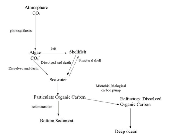
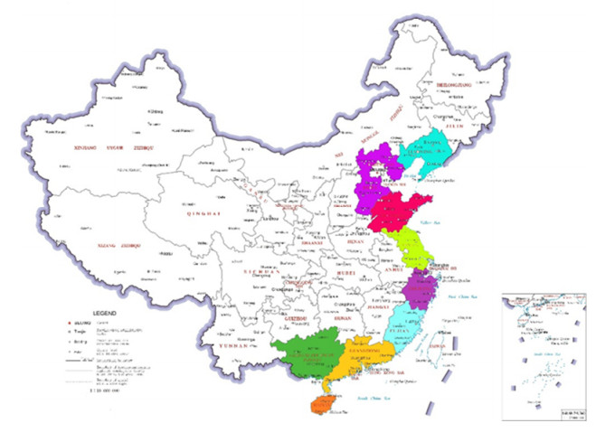
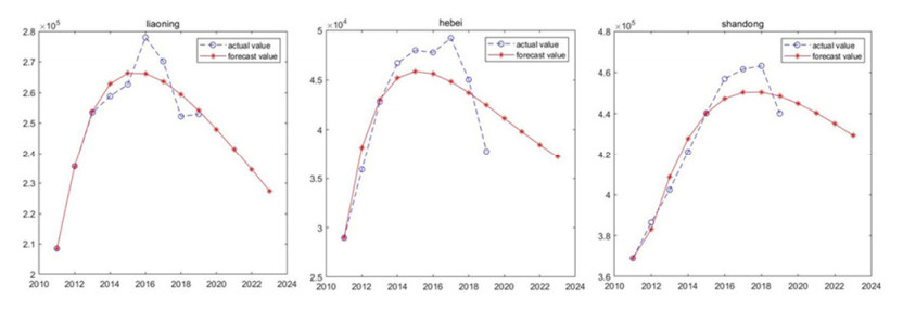
Marine biology carbon sinks function is vital pathway to earned carbon neutrality object. Algae and shellfish can capture CO₂ from atmosphere reducing CO₂ concentration. Therefore, algae and shellfish carbon sink capability investigate and forecast are important problem. The study forecast algae and shellfish carbon sinks capability trend base on 9 China coastal provinces. Fractional order accumulation grey model (FGM) is employed to forecast algae and shellfish carbon sinks capability. The result showed algae and shellfish have huge carbon sinks capability. North coastal provinces algae and shellfish carbon sinks capability trend smoothness. South and east coastal provinces carbon sinks capability trend changed drastically. The research advised coastal provinces defend algae and shellfish population, expand carbon sink capability. Algae and shellfish carbon sink resource will promote environment sustainable develop.
- marine carbon sinks capability,
- algae and shellfish,
- FGM
Citation: Haolei Gu, Kedong Yin. Forecasting algae and shellfish carbon sink capability on fractional order accumulation grey model[J]. Mathematical Biosciences and Engineering, 2022, 19(6): 5409-5427. doi: 10.3934/mbe.2022254

Related Papers:

Abstract

Marine biology carbon sinks function is vital pathway to earned carbon neutrality object. Algae and shellfish can capture CO₂ from atmosphere reducing CO₂ concentration. Therefore, algae and shellfish carbon sink capability investigate and forecast are important problem. The study forecast algae and shellfish carbon sinks capability trend base on 9 China coastal provinces. Fractional order accumulation grey model (FGM) is employed to forecast algae and shellfish carbon sinks capability. The result showed algae and shellfish have huge carbon sinks capability. North coastal provinces algae and shellfish carbon sinks capability trend smoothness. South and east coastal provinces carbon sinks capability trend changed drastically. The research advised coastal provinces defend algae and shellfish population, expand carbon sink capability. Algae and shellfish carbon sink resource will promote environment sustainable develop.

References

[1]	S. Khatiwala, T. Tanhua, S. M. Fletcher, M. Gerber, S. C. Doney, H. D. Graven, et al., Global ocean storage of anthropogenic carbon, Biogeosciences, 10 (2013), 2169–2191. https://doi.org/10.5194/bg-10-2169-2013 doi: 10.5194/bg-10-2169-2013
[2]	J. Wu, B. Li, Spatio-temporal evolutionary characteristics of carbon emissions and carbon sinks of marine industry in China and their time-dependent models, Mar. Policy, 135 (2022), 104879. https://doi.org/10.1016/j.marpol.2021.104879 doi: 10.1016/j.marpol.2021.104879
[3]	T. DeVries, C. L. Quéré, O. Andrews, Decadal trends in the ocean carbon sink, Proc. Natl. Acad. Sci. U. S. A., 116 (2019), 11646–11651. https://doi.org/10.1073/pnas.1900371116 doi: 10.1073/pnas.1900371116
[4]	V. V. S. S. Sarma, M. D. Kumar, T. Saino, Impact of sinking carbon flux on accumulation of deep-ocean carbon in the Northern Indian Ocean, Biogeochemistry, 82 (2007), 89–100. https://doi.org/10.1007/s10533-006-9055-1 doi: 10.1007/s10533-006-9055-1
[5]	M. R. Stukel, L. I. Aluwihare, K. A. Barbeau, A. M. Chekalyuk, R. Goericke, A. J. Miller, et al., Mesoscale ocean fronts enhance carbon export due to gravitational sinksing and subduction, Proc. Natl. Acad. Sci. U. S. A., 114 (2017), 1252–1257. https://doi.org/10.1073/pnas.1609435114 doi: 10.1073/pnas.1609435114
[6]	C. Ma, K. You, D. Ji, W. Ma, F. Li, Primary discussion of a carbon sink in the oceans, J. Ocean Univ. China, 14 (2015), 284–292. https://doi.org/10.1007/s11802-015-2548-6 doi: 10.1007/s11802-015-2548-6
[7]	K. Rehdanz, R. S. J. Tol, P. Wetzel, Ocean carbon sinks and international climate policy, Energy Policy, 34 (2006), 3516–3526. https://doi.org/10.1016/j.enpol.2005.07.015 doi: 10.1016/j.enpol.2005.07.015
[8]	L. Gloege, G. A. McKinley, P. Landschützer, A. R. Fay, T. L. Frölicher, J. C. Fyfe, et al., Quantifying errors in observationally based estimates of ocean carbon sink variability, Global Biogeochem. Cycles, 35 (2021), e2020GB006788. https://doi.org/10.1029/2020GB006788 doi: 10.1029/2020GB006788
[9]	F. Lacroix, T. Ilyina, G. G. Laruelle, P. Regnier, Reconstructing the preindustrial coastal carbon cycle through a global ocean circulation model: was the global continental shelf already both autotrophic and a CO₂ sinks? Global Biogeochem. Cycles, 35 (2021), e2020GB006603. https://doi.org/10.1029/2020GB006603 doi: 10.1029/2020GB006603
[10]	H. J. Jeong, Y. D. Yoo, K. Lee, H. C. Kang, J. S. Kim, K. Y. Kim, Annual carbon retention of a marine-plankton community in the eutrophic masan bay, based on daily measurements, Mar. Biol., 168 (2021), 69. https://doi.org/10.1007/s00227-021-03881-4 doi: 10.1007/s00227-021-03881-4
[11]	A. Olivier, L. L. Vay, S. K. Malham, M. Christie, J. Wilson, S. Allender, et al., Geographical variation in the carbon, nitrogen, and phosphorus content of blue mussels, Mytilus edulis, Mar. Pollut. Bull., 167 (2021), 112291. https://doi.org/10.1016/j.marpolbul.2021.112291 doi: 10.1016/j.marpolbul.2021.112291
[12]	G. K. Vondolia, W. Chen, C. W. Armstrong, M. D. Norling, Bioeconomic modelling of coastal cod and kelp forest interactions: Co-benefits of habitat services, fisheries and carbon sinks, Environ. Resour. Econ., 75 (2020), 25–48. https://doi.org/10.1007/s10640-019-00387-y doi: 10.1007/s10640-019-00387-y
[13]	J. Sui, J. Zhang, S. J. Ren, F. Lin, Organic carbon in the surface sediments from the intensive mariculture zone of sanggou bay: Distribution, seasonal variations and dources, J. Ocean Univ. China, 18 (2019), 985–996. https://doi.org/10.1007/s11802-019-3768-y doi: 10.1007/s11802-019-3768-y
[14]	A. Roura, J. M. Strugnell, Á. Guerra, Á. F. González, A. J. Richardson, Small copepods could channel missing carbon through metazoan predation, Ecol. Evol., 8 (2018), 10868–10878. https://doi.org/10.1002/ece3.4546 doi: 10.1002/ece3.4546
[15]	J. B. Gallagher, Taking stock of mangrove and seagrass blue carbon ecosystems: A perspective for future carbon trading, Borneo J. Mar. Sci. Aquacult., 1 (2017), 71–74. https://doi.org/10.51200/bjomsa.v1i0.994 doi: 10.51200/bjomsa.v1i0.994
[16]	B. D. Schwartzkopf, S. A. Heppell, A feeding-ecology-based approach to evaluating nursery potential of estuaries for black rockfish, Mar. Coastal Fish., 12 (2020), 124–141. https://doi.org/10.1002/mcf2.10115 doi: 10.1002/mcf2.10115
[17]	C. Corinaldesi, S. Canensi, A. D. Anno, M. Tangherlini, I. D. Capua, S. Varrella, et al., Multiple impacts of microplastics can threaten marine habitat-forming species, Commun. Biol., 4 (2021), 431. https://doi.org/10.1038/s42003-021-01961-1 doi: 10.1038/s42003-021-01961-1
[18]	C. Bertolini, I. Bernardini, D. Brigolin, V. Matozzo, M. Milan, R. Pastres, A bioenergetic model to address carbon sequestration potential of shellfish farming: example from Ruditapes philippinarum in the Venice lagoon, ICES J. Mar. Sci., 78 (2021), 2082–2091. https://doi.org/10.1093/icesjms/fsab099 doi: 10.1093/icesjms/fsab099
[19]	J. Guiet, Environmental Impact on Fish Communities in The Global Ocean: A Mechanistic Modeling Approach, 2016.
[20]	J. L. Deng, Control problems of grey systems, Syst. Control Lett., 1 (1982), 288–294. https://doi.org/10.1016/S0167-6911(82)80025-X doi: 10.1016/S0167-6911(82)80025-X
[21]	D. Lei, K. Wu, L. Zhang, W. Li, Q. Liu, Neural ordinary differential grey model and its applications, Expert Syst. Appl., 177 (2021), 114923. https://doi.org/10.1016/j.eswa.2021.114923 doi: 10.1016/j.eswa.2021.114923
[22]	Y. Kang, S. Mao, Y. Zhang, Variable order fractional grey model and its application, Appl. Math. Modell., 97 (2021), 619–635. https://doi.org/10.1016/j.apm.2021.03.059 doi: 10.1016/j.apm.2021.03.059
[23]	W. Xie, M. Pang, W. Wu, C. Liu, C. X. Liu, A Framework for General Conformable Fractional Grey System Models: A Physical Perspective and Its Actual Application, 2021.
[24]	J. Jiang, T. Feng, C. Liu, An improved nonlinear grey bernoulli model based on the whale optimization algorithm and its application, Math. Probl. Eng., 2021 (2021), 6691724. https://doi.org/10.1155/2021/6691724 doi: 10.1155/2021/6691724
[25]	L. Yu, X. Ma, W. Wu, X. Xiang, Y. Wang, B. Zeng, Application of a novel time-delayed power-driven grey model to forecast photovoltaic power generation in the Asia-pacific region, Sustainable Energy Technol. Assess., 44 (2021), 100968. https://doi.org/10.1016/j.seta.2020.100968 doi: 10.1016/j.seta.2020.100968
[26]	Z. Xu, L. Liu, L. Wu, Forecasting the carbon dioxide emissions in 53 countries and regions using a non-equigap grey model, Environ. Sci. Pollut. Res., 28 (2021), 15659–15672. https://doi.org/10.1007/s11356-020-11638-7 doi: 10.1007/s11356-020-11638-7
[27]	J. Wang, P. Du, Quarterly PM2.5 prediction using a novel seasonal grey model and its further application in health effects and economic loss assessment: evidences from Shanghai and Tianjin, China, Nat. Hazards, 107 (2021), 889–909. https://doi.org/10.1007/s11069-021-04614-y doi: 10.1007/s11069-021-04614-y
[28]	Y. Cao, K. Yin, X. Li, C. Zhai, Forecasting CO₂ emissions from Chinese marine fleets using multivariable trend interaction grey model, Appl. Soft Comput., 104 (2021), 107220. https://doi.org/10.1016/j.asoc.2021.107220 doi: 10.1016/j.asoc.2021.107220
[29]	L. Tu, Y. Chen, An unequal adjacent grey forecasting air pollution urban model, Appl. Math. Modell., 99 (2021), 260–275. https://doi.org/10.1016/j.apm.2021.06.025 doi: 10.1016/j.apm.2021.06.025
[30]	S. Ding, R. Li, S. Wu, W. Zhou, Application of a novel structure-adaptative grey model with adjustable time power item for nuclear energy consumption forecasting, Appl. Energy, 298 (2021), 117114. https://doi.org/10.1016/j.apenergy.2021.117114 doi: 10.1016/j.apenergy.2021.117114
[31]	S. Ding, R. Lin, Z. Tao, A novel adaptive discrete grey model with time-varying parameters for long-term photovoltaic power generation forecasting, Energy Convers. Manage., 227 (2021), 113644. https://doi.org/10.1016/j.enconman.2020.113644 doi: 10.1016/j.enconman.2020.113644
[32]	S. Ding, R. Li, S. Wu, A novel composite forecasting framework by adaptive data preprocessing and optimized nonlinear grey bernoulli model for new energy vehicles sales, Commun. Nonlinear Sci. Numer. Simul., 99 (2021), 105847. https://doi.org/10.1016/j.cnsns.2021.105847 doi: 10.1016/j.cnsns.2021.105847
[33]	M. Wang, W. Wang, L. Wu, Application of a new grey multivariate forecasting model in the forecasting of energy consumption in 7 regions of China, Energy, 243 (2022), 123024. https://doi.org/10.1016/j.energy.2021.123024 doi: 10.1016/j.energy.2021.123024
[34]	B. Zeng, H. Li, Prediction of coalbed methane production in China based on an optimized grey system model, Energy Fuels, 35 (2021), 4333−4344. https://doi.org/10.1021/acs.energyfuels.0c04195 doi: 10.1021/acs.energyfuels.0c04195
[35]	B. Zeng, M. Zhou, X. Liu, Z. Zhang, Application of a new grey prediction model and grey average weakening buffer operator to forecast China's shale gas output, Energy Rep., 6 (2020), 1608–1618. https://doi.org/10.1016/j.egyr.2020.05.021 doi: 10.1016/j.egyr.2020.05.021
[36]	Q. Tang, J. Zhang, J. Fang, Shellfish and seaweed mariculture increase atmospheric CO₂ absorption by coastal ecosystems, Mar. Ecol. Prog. Ser., 424 (2011), 97–104. https://doi.org/10.3354/meps08979 doi: 10.3354/meps08979
[37]	B. E. Lapointe, M. M. Littler, D. S. Littler, A comparison of nutrient-limited productivity and physiological state in macroalgae from a caribbean barrier reef and mangrove ecosystem, Aquat. Bot., 28 (1987), 243–255. https://doi.org/10.1016/0304-3770(87)90003-9 doi: 10.1016/0304-3770(87)90003-9
[38]	G. Rosenberg, T. A. Probyn, K. H. Mann, Nutrient uptake and growth kinetics in brown seaweeds: response to continuous and single additions of ammonium, J. Exp. Mar. Biol. Ecol., 80 (1984), 125–146. https://doi.org/10.1016/0022-0981(84)90008-X doi: 10.1016/0022-0981(84)90008-X
[39]	D. Xu, G. Bewnn, L. Xu, X. W. Zhang, X. Fan, W. T. Han, et al., Ocean acidification increases iodine accumulation in kelp-based coastal food webs, Global Change Biol., 25 (2019), 629–639. https://doi.org/10.1111/gcb.14467 doi: 10.1111/gcb.14467
[40]	L. Wu, S. Liu, L. Yao, S. Yan, D. Liu, Grey system model with the fractional order accumulation, Commun. Nonlinear Sci. Numer. Simul., 18 (2013), 1775–1785. https://doi.org/10.1016/j.cnsns.2012.11.017 doi: 10.1016/j.cnsns.2012.11.017

Reader Comments

Your name:*

Email:*
© 2022 the Author(s), licensee AIMS Press. This is an open access article distributed under the terms of the Creative Commons Attribution License (http://creativecommons.org/licenses/by/4.0)