Numerical investigations of the nonlinear smoke model using the Gudermannian neural networks

Zulqurnain Sabir; Muhammad Asif Zahoor Raja; Abeer S. Alnahdi; Mdi Begum Jeelani; M. A. Abdelkawy; Zulqurnain Sabir; Muhammad Asif Zahoor Raja; Abeer S. Alnahdi; Mdi Begum Jeelani; M. A. Abdelkawy

doi:10.3934/mbe.2022018

Mathematical Biosciences and Engineering

2022, Volume 19, Issue 1: 351-370. doi: 10.3934/mbe.2022018

Previous Article Next Article

Research article

Numerical investigations of the nonlinear smoke model using the Gudermannian neural networks

1.
Department of Mathematics and Statistics, Hazara University, Mansehra, Pakistan
2.
Future Technology Research Center, National Yunlin University of Science and Technology, 123 University Road, Section 3, Douliou, Yunlin 64002, Taiwan, R.O.C
3.
Department of Mathematics and Statistics, Faculty of Science, Imam Mohammad Ibn Saud Islamic University, Riyadh, Saudi Arabia
4.
Department of Mathematics, Faculty of Science, Beni-Suef University, Beni-Suef, Egypt

Academic Editor: Zhi-Cheng Wang

Received: 25 August 2021 Accepted: 17 October 2021 Published: 15 November 2021

These investigations are to find the numerical solutions of the nonlinear smoke model to exploit a stochastic framework called gudermannian neural works (GNNs) along with the optimization procedures of global/local search terminologies based genetic algorithm (GA) and interior-point algorithm (IPA), i.e., GNNs-GA-IPA. The nonlinear smoke system depends upon four groups, temporary smokers, potential smokers, permanent smokers and smokers. In order to solve the model, the design of fitness function is presented based on the differential system and the initial conditions of the nonlinear smoke system. To check the correctness of the GNNs-GA-IPA, the obtained results are compared with the Runge-Kutta method. The plots of the weight vectors, absolute error and comparison of the results are provided for each group of the nonlinear smoke model. Furthermore, statistical performances are provided using the single and multiple trial to authenticate the stability and reliability of the GNNs-GA-IPA for solving the nonlinear smoke system.
- Gudermannain neural networks,
- nonlinear smoke model,
- Runge-Kutta,
- active-set algorithm,
- genetic algorithms,
- numerical results
Citation: Zulqurnain Sabir, Muhammad Asif Zahoor Raja, Abeer S. Alnahdi, Mdi Begum Jeelani, M. A. Abdelkawy. Numerical investigations of the nonlinear smoke model using the Gudermannian neural networks[J]. Mathematical Biosciences and Engineering, 2022, 19(1): 351-370. doi: 10.3934/mbe.2022018

Related Papers:

Abstract

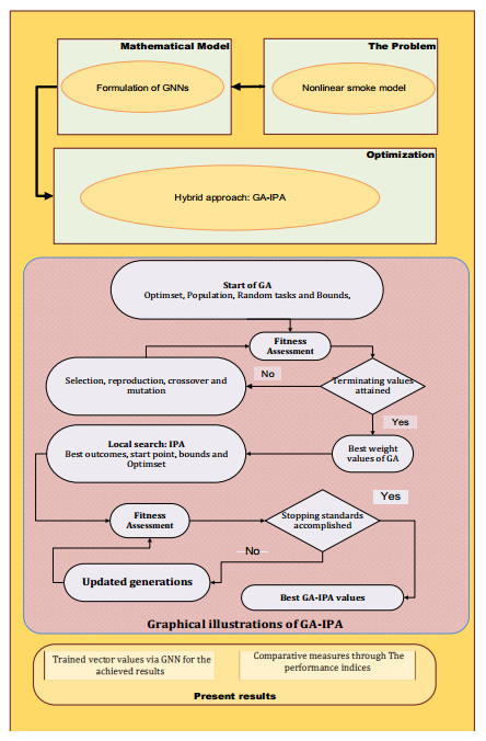
These investigations are to find the numerical solutions of the nonlinear smoke model to exploit a stochastic framework called gudermannian neural works (GNNs) along with the optimization procedures of global/local search terminologies based genetic algorithm (GA) and interior-point algorithm (IPA), i.e., GNNs-GA-IPA. The nonlinear smoke system depends upon four groups, temporary smokers, potential smokers, permanent smokers and smokers. In order to solve the model, the design of fitness function is presented based on the differential system and the initial conditions of the nonlinear smoke system. To check the correctness of the GNNs-GA-IPA, the obtained results are compared with the Runge-Kutta method. The plots of the weight vectors, absolute error and comparison of the results are provided for each group of the nonlinear smoke model. Furthermore, statistical performances are provided using the single and multiple trial to authenticate the stability and reliability of the GNNs-GA-IPA for solving the nonlinear smoke system.

References

[1]	B. Hipple, H. Lando, J. Klein, J. Winickoff, Global teens and tobacco: a review of the globalization of the tobacco epidemic, Curr. Probl. Pediatr. Adolesc. Health Care, 41 (2011), 216–230. doi: 10.1016/j.cppeds.2011.02.010. doi: 10.1016/j.cppeds.2011.02.010
[2]	World Health Organization, WHO Report on the Global Tobacco Epidemic, 2009: Implementing Smoke-free Environments: Executive Summary, 2009. Available from: http://apps.who.int/iris/bitstream/handle/10665/70429/WHO_NMH_TFI_09.1_eng.pdf;sequene=1.
[3]	C. Castillo-Garsow, G. Jordán-Salivia, A. Rodriguez-Herrera, Mathematical models for the dynamics of tobacco use, recovery and relapse, Garsow, (1997). Available from: https://hdl.handle.net/1813/32095.
[4]	O. Sharomi, A. B. Gumel, Curtailing smoking dynamics: a mathematical modeling approach, Appl. Math. Comput., 195 (2008), 475–499. doi: 10.1016/j.amc.2007.05.012. doi: 10.1016/j.amc.2007.05.012
[5]	Z. Sabir, M. Umar, M. A. Z. Raja, D. Baleanu, Applications of Gudermannian neural network for solving the SITR fractal system, Fractals, (2021). doi: 10.1142/S0218348X21502509. doi: 10.1142/S0218348X21502509
[6]	Z. Sabir, M. A. Z. Raja, D. Baleanu, R. Sadat, M. R. Ali, Investigations of nonlinear induction motor model using the Gudermannian neural networks, Therm. Sci., (2021). doi: 10.2298/TSCI210508261S. doi: 10.2298/TSCI210508261S
[7]	K. Nisar, Z, Sabir, M. A. Z. Raja, A. A. A. Ibrahim, D. B. Rawat, Evolutionary integrated heuristic with Gudermannian neural networks for second kind of Lane-Emden nonlinear singular models, Appl. Sci., 11 (2021), 4725. doi: 10.3390/app11114725. doi: 10.3390/app11114725
[8]	Z. Sabir, M. A. Z. Raja, A. Arbi, G. C. Altamirano, J. Cao, Neuro-swarms intelligent computing using Gudermannian kernel for solving a class of second order Lane-Emden singular nonlinear model, AIMS Math., 6 (2021), 2468–2485. doi: 10.3934/math.2021150. doi: 10.3934/math.2021150
[9]	M. Higazy, A. M. S. Mahdy, N. H. Sweilam, Approximate solutions for solving nonlinear fractional order smoking model, Alexandria Eng. J., 59 (2020), 739–752. doi: 10.1016/j.aej.2020.01.049. doi: 10.1016/j.aej.2020.01.049
[10]	A. M. S. Mahdy, Numerical studies for solving fractional integro-differential equations, J. Ocean Eng. Sci., 3 (2018), 127–132. doi: 10.1016/j.joes.2018.05.004. doi: 10.1016/j.joes.2018.05.004
[11]	A. M. S. Mahdy, M. Higazy, K. A. Gepreel, A. A. A. El-dahdouh, Optimal control and bifurcation diagram for a model nonlinear fractional SIRC, Alexandria Eng. J., 59 (2020), 3481–3501. doi: 10.1016/j.aej.2020.05.028. doi: 10.1016/j.aej.2020.05.028
[12]	J. Zhang, C. Chen, X. Yang, Y. Chu, Z. Xia, Efficient, non-iterative, and second-order accurate numerical algorithms for the anisotropic Allen-Cahn equation with precise nonlocal mass conservation, J. Comput. Appl. Math., 363 (2020), 444–463. doi: 10.1016/j.cam.2019.05.003. doi: 10.1016/j.cam.2019.05.003
[13]	A. M. S. Mahdy, K. Lotfy, W. Hassan, A. A. El-Bary, Analytical solution of magneto-photothermal theory during variable thermal conductivity of a semiconductor material due to pulse heat flux and volumetric heat source, Waves Random Complex Media, (2020), 1–18. doi: 10.1080/17455030.2020.1717673. doi: 10.1080/17455030.2020.1717673
[14]	K. Lotfy, Effect of variable thermal conductivity during the photothermal diffusion process of semiconductor medium, Silicon, 11 (2019), 1863–1873. doi: 10.1007/s12633-018-0005-z. doi: 10.1007/s12633-018-0005-z
[15]	I. Ahmad, H. Ilyas, M. A. Z. Raja, Z. Khan, M. Shoaib, Stochastic numerical computing with Levenberg-Marquardt backpropagation for performance analysis of heat sink of functionally graded material of the porous fin, Surf. Interfaces, 26 (2021), 101403. doi: 10.1016/j.surfin.2021.101403. doi: 10.1016/j.surfin.2021.101403
[16]	H. Ilyas, A. Iftikhar, M. A. Z. Raja, M. B. Tahir, M Shoaib, Intelligent computing for the dynamics of fluidic system of electrically conducting Ag/Cu nanoparticles with mixed convection for hydrogen possessions, Int. J. Hydrogen Energy, 46 (2021), 4947–4980. doi: 10.1016/j.ijhydene.2020.11.097. doi: 10.1016/j.ijhydene.2020.11.097
[17]	T. N. Cheema, M. A. Z. Raja, A. Iftikhar, S. Naz, M. Shoaib, Intelligent computing with Levenberg-Marquardt artificial neural networks for nonlinear system of COVID-19 epidemic model for future generation disease control, Eur. Phys. J. Plus, 135 (2020), 1–35. doi: 10.1140/epjp/s13360-020-00910-x. doi: 10.1140/epjp/s13360-020-00910-x
[18]	Z. Sabir, M. A.Z. Raja, M. Umar, M. Shoaib, Design of neuro-swarming-based heuristics to solve the third-order nonlinear multi-singular Emden-Fowler equation, Eur. Phys. J. Plus, 135 (2020), 1–17. doi: 10.1140/epjp/s13360-020-00424-6. doi: 10.1140/epjp/s13360-020-00424-6
[19]	Z. Sabir, M. A. Z. Raja, M. Umar, M. Shoaib, Neuro-swarm intelligent computing to solve the second-order singular functional differential model, Eur. Phys. J. Plus, 135 (2020), 474. doi: 10.1140/epjp/s13360-020-00440-6. doi: 10.1140/epjp/s13360-020-00440-6
[20]	M. Umar, Z, Sabir, M. A. Z. Raja, Y. G. Sánchez, A stochastic numerical computing heuristic of SIR nonlinear model based on dengue fever, Results Phys., 19 (2020), 103585. doi: 10.1016/j.rinp.2020.103585. doi: 10.1016/j.rinp.2020.103585
[21]	A. K. Kiani, W. U. Khan, M. A. Z. Raja, Y. He, Z. Sabir, M. Shoaib, Intelligent backpropagation networks with bayesian regularization for mathematical models of environmental economic systems, Sustainability, 13 (2021), 9537. doi: 10.3390/su13179537. doi: 10.3390/su13179537
[22]	M. Umar, Z. Sabir, M. A. Z. Raja, Intelligent computing for numerical treatment of nonlinear prey-predator models, Appl. Soft Comput., 80 (2019), 506–524. doi: 10.1016/j.asoc.2019.04.022. doi: 10.1016/j.asoc.2019.04.022
[23]	Z. Sabir, M. A. Manzar, M. A. Z. Raja, M. Sheraz, A. M. Wazwaz, Neuro-heuristics for nonlinear singular Thomas-Fermi systems, Appl. Soft Comput., 65 (2018), 152–169. doi: 10.1016/j.asoc.2018.01.009. doi: 10.1016/j.asoc.2018.01.009
[24]	M. Umar, M. A. Z. Raja, Z. Sabir, A. S. Alwabli, M. Shoaib, A stochastic computational intelligent solver for numerical treatment of mosquito dispersal model in a heterogeneous environment, Eur. Phys. J. Plus, 135 (2020), 1–23. doi: 10.1140/epjp/s13360-020-00557-8. doi: 10.1140/epjp/s13360-020-00557-8
[25]	M. A. Z. Raja, U, Muhammad, S, Zulqurnain, K. J. Ali, B. Dumitru, A new stochastic computing paradigm for the dynamics of nonlinear singular heat conduction model of the human head, Eur. Physical J. Plus, 133 (2018), 364. doi: 10.1140/epjp/s13360-020-00557-8. doi: 10.1140/epjp/s13360-020-00557-8
[26]	Z. Sabir, M. A. Z. Raja, M. Shoaib, J. F. G. Aguilar, FMNEICS: fractional Meyer neuro-evolution-based intelligent computing solver for doubly singular multi-fractional order Lane-Emden system, Comput. Appl. Math., 39 (2020), 1–18. doi: 10.1007/s40314-020-01350-0. doi: 10.1007/s40314-020-01350-0
[27]	M. Umar, Z. Sabir, M. Asif, Z. Raja, YG Sánchez, A stochastic intelligent computing with neuro-evolution heuristics for nonlinear SITR system of novel COVID-19 dynamics, Symmetry, 12 (2020), 1628. doi: 10.3390/sym12101628. doi: 10.3390/sym12101628
[28]	W. Han, B. Hua, X. Ruan, Genetic algorithm-driven discovery of unexpected thermal conductivity enhancement by disorder, Nano Energy, 71 (2020), 104619. doi: 10.1016/j.nanoen.2020.104619. doi: 10.1016/j.nanoen.2020.104619
[29]	S. L. Podvalny, M. I. Chizhov, P. Y. Gusev, K. Y. Gusev, The crossover operator of a genetic algorithm as applied to the task of a production planning, Procedia Comput. Sci., 150 (2019), 603–608. doi: 10.1016/j.procs.2019.02.100. doi: 10.1016/j.procs.2019.02.100
[30]	M. M. Gani, M. S. Islam, M. A. Ullah, Optimal PID tuning for controlling the temperature of electric furnace by genetic algorithm, SN Appl. Sci., 1 (2019), 1–8. doi: 10.1007/s42452-019-0929-y. doi: 10.1007/s42452-019-0929-y
[31]	S. Parinam, M. Kumar, N. Kumari, V. Karar, A. L. Sharma, An improved optical parameter optimisation approach using Taguchi and genetic algorithm for high transmission optical filter design, Optik, 182 (2019), 382–392. doi: 10.1016/j.ijleo.2018.12.189. doi: 10.1016/j.ijleo.2018.12.189
[32]	M. Hajipour, K. Etminani, Z. Rahmatinejad, M. Soltani, K. Etemad, S. Eslami, et al., A predictive model for mortality of patients with thalassemia using logistic regression model and genetic algorithm, Int. J. Health Stud., 4 (2018), 21–26. doi: 10.22100/ijhs.v4i3.523. doi: 10.22100/ijhs.v4i3.523
[33]	J. Wambacq, J. Ulloa, G. Lombaert, S. Franois, Interior-point methods for the phase-field approach to brittle and ductile fracture, Comput. Methods Appl. Mech. Eng., 375 (2021), 113612. doi: 10.1016/j.cma.2020.113612. doi: 10.1016/j.cma.2020.113612
[34]	A. Zanelli, A. Domahidi, J. Jerez, M. Morari, FORCES NLP: an efficient implementation of interior-point methods for multistage nonlinear nonconvex programs, Int. J. Control, 93 (2020), 13–29. doi: 10.1080/00207179.2017.1316017. doi: 10.1080/00207179.2017.1316017
[35]	M. Umar, Z. Sabir, M. A. Z. Raja, F. Amin, Y. G. Sanchez, Integrated neuro-swarm heuristic with interior-point for nonlinear SITR model for dynamics of novel COVID-19, Alexandria Eng. J., 60 (2021), 2811–2824. doi: 10.1016/j.aej.2021.01.043. doi: 10.1016/j.aej.2021.01.043
[36]	J. Bleyer, Advances in the simulation of viscoplastic fluid flows using interior-point methods, Comput. Methods Appl. Mech. Eng., 330 (2018), 368–394. doi: 10.1016/j.cma.2017.11.006. doi: 10.1016/j.cma.2017.11.006
[37]	J. Kardoš, D. Kourounis, O. Schenk, Two-level parallel augmented schur complement interior-point algorithms for the solution of security constrained optimal power flow problems, IEEE Trans. Power Syst., 35 (2019), 1340–1350. doi: 10.1109/TPWRS.2019.2942964. doi: 10.1109/TPWRS.2019.2942964
[38]	M. Umar, Z. Sabir, M. A. Z. Raja, J. F. Gómez Aguilar, F. Amin, M. Shoaib, Neuro-swarm intelligent computing paradigm for nonlinear HIV infection model with CD4+ T-cells, Math. Comput. Simul., (2021). doi: 10.1016/j.matcom.2021.04.008. doi: 10.1016/j.matcom.2021.04.008
[39]	Z. Sabir, M. A. Z. Raja, C. M. Khalique, C. Unlu, Neuro-evolution computing for nonlinear multi-singular system of third order Emden-Fowler equation, Math. Comput. Simul., 185 (2021), 799–812. doi: 10.1016/j.matcom.2021.02.004. doi: 10.1016/j.matcom.2021.02.004
[40]	M. Shoaib, M. A. Z. Raja, M. A. R. Khan, I. Farhat, S. E. Awan, Neuro-computing networks for entropy generation under the influence of MHD and thermal radiation, Surf. Interfaces, (2021), 101243. doi: 10.1016/j.surfin.2021.101243. doi: 10.1016/j.surfin.2021.101243
[41]	Z. Sabir, M. A. Z. Raja, J. L. G. Guirao, M. Shoaib, A novel design of fractional Meyer wavelet neural networks with application to the nonlinear singular fractional Lane-Emden systems, Alexandria Eng. J., 60 (2021), 2641–2659. doi: 10.1016/j.aej.2021.01.004. doi: 10.1016/j.aej.2021.01.004

Reader Comments

Your name:*

Email:*
© 2022 the Author(s), licensee AIMS Press. This is an open access article distributed under the terms of the Creative Commons Attribution License (http://creativecommons.org/licenses/by/4.0)