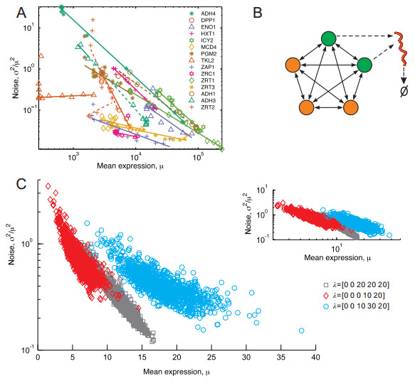
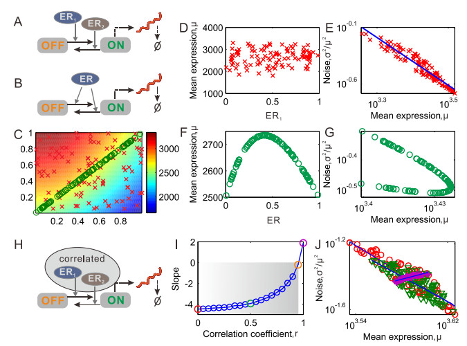
Gene transcription in single cells is inherently a probabilistic process. The relationship between variance ($ \sigma^{2} $) and mean expression ($ \mu $) is of paramount importance for investigations into the evolutionary origins and consequences of noise in gene expression. It is often formulated as $ \log \left({{{\sigma}^{2}}}/{{{\mu}^{2}}}\; \right) = \beta\log\mu+\log\alpha $, where $ \beta $ is a key parameter since its sign determines the qualitative dependence of noise on mean. We reveal that the sign of $ \beta $ is controlled completely by external regulation, but independent of promoter structure. Specifically, it is negative if regulators as stochastic variables are independent but positive if they are correlated. The essential mechanism revealed here can well interpret diverse experimental phenomena underlying expression noise. Our results imply that external regulation rather than promoter sequence governs the mean-noise relationship.
Citation: Meiling Chen, Tianshou Zhou, Jiajun Zhang. Correlation between external regulators governs the mean-noise relationship in stochastic gene expression[J]. Mathematical Biosciences and Engineering, 2021, 18(4): 4713-4730. doi: 10.3934/mbe.2021239
Gene transcription in single cells is inherently a probabilistic process. The relationship between variance ($ \sigma^{2} $) and mean expression ($ \mu $) is of paramount importance for investigations into the evolutionary origins and consequences of noise in gene expression. It is often formulated as $ \log \left({{{\sigma}^{2}}}/{{{\mu}^{2}}}\; \right) = \beta\log\mu+\log\alpha $, where $ \beta $ is a key parameter since its sign determines the qualitative dependence of noise on mean. We reveal that the sign of $ \beta $ is controlled completely by external regulation, but independent of promoter structure. Specifically, it is negative if regulators as stochastic variables are independent but positive if they are correlated. The essential mechanism revealed here can well interpret diverse experimental phenomena underlying expression noise. Our results imply that external regulation rather than promoter sequence governs the mean-noise relationship.

| [1] |
A. Sanchez, S. Choubey, J. Kondev, Regulation of noise in gene expression, Annu. Rev. Biophys., 42 (2013), 469–491. doi: 10.1146/annurev-biophys-083012-130401

|
| [2] |
M. Kaern, T. C. Elston, W. J. Blake, J. J. Collins, Stochasticity in gene expression: from theories to phenotypes, Nat. Rev. Genet., 6 (2005), 451–464. doi: 10.1038/nrg1615
|
| [3] |
J. M. Raser, E. K. O'Shea, Control of Stochasticity in eukaryotic gene expression, Science, 304 (2004), 1811–1814. doi: 10.1126/science.1098641
|
| [4] |
W. J. Blake, G. Balazsi, M. A. Kohanski, F. J. Isaacs, K. F. Murphy, Y. Kuang, et al., Phenotypic consequences of promoter-mediated transcriptional noise, Mol. Cell, 24 (2006), 853–865. doi: 10.1016/j.molcel.2006.11.003
|
| [5] |
N. Q. Balaban, J. Merrin, R. Chait, L. Kowalik, S. Leibler, Bacterial persistence as a phenotypic switch, Science, 305 (2004), 1622–1625. doi: 10.1126/science.1099390
|
| [6] |
H. H. Chang, M. Hemberg, M. Barahona, D. E. Ingber, S. Huang, Transcriptome-wide noise controls lineage choice in mammalian progenitor cells, Nature, 453 (2008), 544–547. doi: 10.1038/nature06965
|
| [7] |
A. Raj, S. A. Rifkin, E. Andersen, A Van Oudenaarden, Variability in gene expression underlies incomplete penetrance, Nature, 463 (2010), 913–918. doi: 10.1038/nature08781
|
| [8] |
G. Hornung, R. Bar-Ziv, D. Rosin, N. Tokuriki, D. S. Tawfik, M. Oren, et al., Noise-mean relationship in mutated promoters, Genome Res., 22 (2012), 2409–2417. doi: 10.1101/gr.139378.112
|
| [9] |
A. Sanchez, I. Golding, Genetic determinants and cellular constraints in noisy gene expression, Science, 342 (2013), 1188–1193. doi: 10.1126/science.1242975
|
| [10] |
L. B. Carey, D. Van Dijk, P. M. Sloot, J. A. Kaandorp, E. Segal, Promoter sequence determines the relationship between expression level and noise, PLoS Biol., 11 (2013), e1001528. doi: 10.1371/journal.pbio.1001528
|
| [11] |
F. L. M. Vallania, M. Sherman, Z. Goodwin, I. Mogno, B. A. Cohen, R. D. Mitra, Origin and consequences of the relationship between protein mean and variance, PLoS ONE, 9 (2014), e102202. doi: 10.1371/journal.pone.0102202
|
| [12] |
S. S. Dey, J. E. Foley, P. Limsirichai, D. V. Schaffer, A. P. Arkin, Orthogonal control of expression mean and variance by epigenetic features at different genomic loci, Mol. Syst. Biol., 11 (2015), 806. doi: 10.15252/msb.20145704
|
| [13] |
R. D. Dar, S. M. Shaffer, A. Singh, B. S. Razooky, M. L. Simpson, A. Raj, et al., Transcriptional bursting explains the noise-versus-mean relationship in mRNA and protein levels, PLoS ONE, 11 (2016), e0158298. doi: 10.1371/journal.pone.0158298
|
| [14] |
R. D. Dar, N. N. Hosmane, M. R. Arkin, R. F. Siliciano, L. S. Weinberger, Screening for noise in gene expression identifies drug synergies, Science, 344 (2014), 1392–1396. doi: 10.1126/science.1250220
|
| [15] |
R. D. Dar, B. S. Razooky, A. Singh, T. V. Trimeloni, J. M. McCollum, C. D. Cox, et al., Transcriptional burst frequency and burst size are equally modulated across the human genome, Proc. Natl. Acad. Sci. USA, 109 (2012), 17454–17459. doi: 10.1073/pnas.1213530109
|
| [16] |
A. Singh, B. Razooky, C. D. Cox, M. L. Simpson, L. S.Weinberger, Transcriptional bursting from the HIV-1 promoter is a significant source of stochastic noise in HIV-1 gene expression, Biophys. J., 98 (2010), L32–L34. doi: 10.1016/j.bpj.2010.03.001
|
| [17] | K. Franz, A. Singh, L. S. Weinberger, Lentiviral vectors to study stochastic noise in gene expression, Methods Enzymol., 497 (2011), 603622. |
| [18] |
R. Skupsky, J. C. Burnett, J. E. Foley, D. V. Schaffer, A. P. Arkin, HIV promoter integration site primarily modulates transcriptional burst size rather than frequency, PLoS Comput. Biol., 6 (2010), e1000952. doi: 10.1371/journal.pcbi.1000952
|
| [19] |
A. Bar-Even, J. Paulsson, N. Maheshri, M. Carmi, E. O'Shea, Y. Pilpel, et al., Noise in protein expression scales with natural protein abundance, Nat. Genet., 38 (2006), 636–643. doi: 10.1038/ng1807
|
| [20] |
L. H. So, A. Ghosh, C. Zong, L. A. Sepúlveda, R. Segev, I. Golding, General properties of transcriptional time series in Escherichia coli, Nat. Genet., 43 (2011), 554–560. doi: 10.1038/ng.821
|
| [21] |
Y. Taniguchi, P. J. Choi, G. W. Li, H. Chen, M. Babu, J. Hearn, et al., Quantifying E. coli proteome and transcriptome with single-molecule sensitivity in single cells, Science, 329 (2010), 533–538. doi: 10.1126/science.1188308
|
| [22] |
B. Zoller, S. C. Little, T. Gregor, Diverse spatial expression patterns emerge from unified kinetics of transcriptional bursting, Cell, 175 (2018), 835–847. doi: 10.1016/j.cell.2018.09.056
|
| [23] |
J. Rodriguez, G. Ren, C. R. Day, K. Zhao, C. C. Chow, D. R. Larson, Intrinsic dynamics of a human gene reveal the basis of expression heterogeneity, Cell, 176 (2019), 213–226. doi: 10.1016/j.cell.2018.11.026
|
| [24] |
J. J. Zhang, T. S. Zhou, Promoter-mediated transcriptional dynamics, Biophys. J., 106 (2014), 479–488. doi: 10.1016/j.bpj.2013.12.011
|
| [25] |
J. Paulsson, Summing up the noise in gene networks, Nature, 427 (2004), 415–418. doi: 10.1038/nature02257
|
| [26] |
T. B. Kepler, T. C. Elston, Stochasticity in transcriptional regulation: Origins, consequences, and mathematical representations, Biophys. J., 81 (2001), 3116–3136. doi: 10.1016/S0006-3495(01)75949-8
|
| [27] |
J. Peccoud, B. Ycart, Markovian modeling of gene-product synthesis, Theor. Popul. Biol., 48 (1995), 222–234. doi: 10.1006/tpbi.1995.1027
|
| [28] |
A. Raj, C. S. Peskin, D. Tranchina, D. Y. Vargas, S. Tyagi, Stochastic mRNA synthesis in mammalian cells, PLoS Biol., 4 (2006), e309. doi: 10.1371/journal.pbio.0040309
|
| [29] |
A. Schwabe, K. N. Rybakova, F. J. Bruggeman, Transcription stochasticity of complex gene regulation models, Biophys. J., 103 (2012), 1152–1161. doi: 10.1016/j.bpj.2012.07.011
|
| [30] |
J. J. Zhang, T. S. Zhou, Stationary moments, distribution conjugation and phenotypic regions in stochastic gene transcription, Math. Biosci. Eng., 16 (2019), 6134–6166. doi: 10.3934/mbe.2019307
|
| [31] | P. S. Swain, M. B. Elowitz, E. D. Siggia, Intrinsic and extrinsic contributions to stochasticity in gene expression, Proc. Natl. Acad. Sci. USA, 999 (2002), 12795–12800. |
| [32] |
T. Q. Liu, J. J. Zhang, T. S. Zhou, Effect of interaction between chromatin loops on cell-to-cell variability in gene expression, PLoS Comput. Biol., 12 (2016), e1004917. doi: 10.1371/journal.pcbi.1004917
|
| [33] |
J. M. Pedraza, J. Paulsson, Effects of molecular memory and bursting on fluctuations in gene expression, Science, 319 (2008), 339–343. doi: 10.1126/science.1144331
|
| [34] |
T. Jia, R. V. Kulkarni, Intrinsic noise in stochastic models of gene expression with molecular memory and bursting, Phys. Rev. Lett., 106 (2011), 058102. doi: 10.1103/PhysRevLett.106.058102
|
| [35] |
J. J. Zhang, T. S. Zhou, Markovian approaches to modeling intracellular reaction processes with molecular memory, Proc. Natl. Acad. Sci. USA, 116 (2019), 23542–23550. doi: 10.1073/pnas.1913926116
|
| [36] |
N. Kumar, A. Singh, R. V. Kulkarni, Transcriptional bursting in gene expression analytical results for general stochastic models, PLoS. Comput. Biol., 11 (2015), e1004292. doi: 10.1371/journal.pcbi.1004292
|
| [37] | R. Milo, R. Phillips, emphCell biology by the numbers, Garland Science, (2015). |
| [38] |
J. Holehouse, Z. Cao, R. Grima, Stochastic modeling of autoregulatory genetic feedback loops: A review and comparative study, Biophys. J., 118 (2020), 1517–1525. doi: 10.1016/j.bpj.2020.02.016
|
| [39] |
V. Shahrezaei, P. S. Swain, Analytical distributions for stochastic gene expression, Proc. Natl. Acad. Sci. USA, 105 (2008), 17256–17261. doi: 10.1073/pnas.0803850105
|
| [40] |
N. Friedman, L. Cai, X. S. Xie, Linking stochastic dynamics to population distribution: an analytical framework of gene expression, Phys. Rev. Lett., 97 (2006), 168302. doi: 10.1103/PhysRevLett.97.168302
|
| [41] |
Y. Liu, A. Beyer, R. Aebersold, On the dependency of cellular protein levels on mRNA abundance, Cell, 165 (2016), 535–550. doi: 10.1016/j.cell.2016.03.014
|
| [42] |
J. J. Zhang, Q. Nie, T. S. Zhou, A moment-convergence method for stochastic analysis of biochemical reaction networks, J. Chem. Phys., 144 (2016), 194109. doi: 10.1063/1.4950767
|
| [43] |
L. Liu, B. R. K. Kashyap, J. G. C. Templeton, On the $G{{I}^{X}}/G/\infty $ system, J. Appl. Probab., 27 (1990), 671–683. doi: 10.2307/3214550
|
| [44] |
D. Nicolas, B. Zoller, D. M. Suter, F. Naef, Modulation of transcriptional burst frequency by histone acetylation, Proc. Natl. Acad. Sci. USA, 115 (2018), 7153–7158. doi: 10.1073/pnas.1722330115
|
| [45] |
S. Wu, K. Li, Y. Li, T. Zhao, T. Li, Y. F. Yang, et al., Independent regulation of gene expression level and noise by histone modifications, PLoS Comput. Biol., 13 (2017), e1005585. doi: 10.1371/journal.pcbi.1005585
|
| [46] |
X. Chen, J. Zhang, The genomic landscape of position effects on protein expression level and noise in yeast, Cell Syst., 2 (2016), 347–35 doi: 10.1016/j.cels.2016.03.009
|
| [47] |
J. M. Schmiedel, L. B. Carey, B. Lehner, Empirical mean-noise fitness landscapes reveal the fitness impact of gene expression noise, Nat. Commun., 10 (2019), 3180. doi: 10.1038/s41467-019-11116-w
|
| [48] |
J. Paulsson, Models of stochastic gene expression, Phys. Life. Rev., 2 (2005), 157–175. doi: 10.1016/j.plrev.2005.03.003
|
| [49] |
C. H. L. Beentjes, R. Perez-Carrasco, R. Grima, Exact solution of stochastic gene expression models with bursting, cell cycle and replication dynamics, Phys. Rev. E, 101 (2020), 032403. doi: 10.1103/PhysRevE.101.032403
|
| [50] |
B. H. Qiu, T. S. Zhou, J. J. Zhang, Stochastic fluctuations in apoptotic threshold of tumour cells can enhance apoptosis and combat fractional killing, R. Soc. Open. Sci., 7 (2020), 190462. doi: 10.1098/rsos.190462
|
Figures(2)

Meiling Chen, Tianshou Zhou, Jiajun Zhang. Correlation between external regulators governs the mean-noise relationship in stochastic gene expression[J]. Mathematical Biosciences and Engineering, 2021, 18(4): 4713-4730. doi: 10.3934/mbe.2021239


 DownLoad: