Conformation and mechanics of the polymeric cuff of artificial urinary sphincter

Arturo Nicola Natali; Chiara Giulia Fontanella; Silvia Todros; Piero G. Pavan; Simone Carmignato; Filippo Zanini; Emanuele Luigi Carniel; Arturo Nicola Natali; Chiara Giulia Fontanella; Silvia Todros; Piero G. Pavan; Simone Carmignato; Filippo Zanini; Emanuele Luigi Carniel

doi:10.3934/mbe.2020216

Mathematical Biosciences and Engineering

2020, Volume 17, Issue 4: 3894-3908. doi: 10.3934/mbe.2020216

Previous Article Next Article

Research article Special Issues

Conformation and mechanics of the polymeric cuff of artificial urinary sphincter

1.
Department of Industrial Engineering, University of Padova, Italy
2.
Centre for Mechanics of Biological Materials, University of Padova, Italy
3.
Department of Management and Engineering, University of Padova, Italy

Received: 09 March 2020 Accepted: 17 May 2020 Published: 25 May 2020

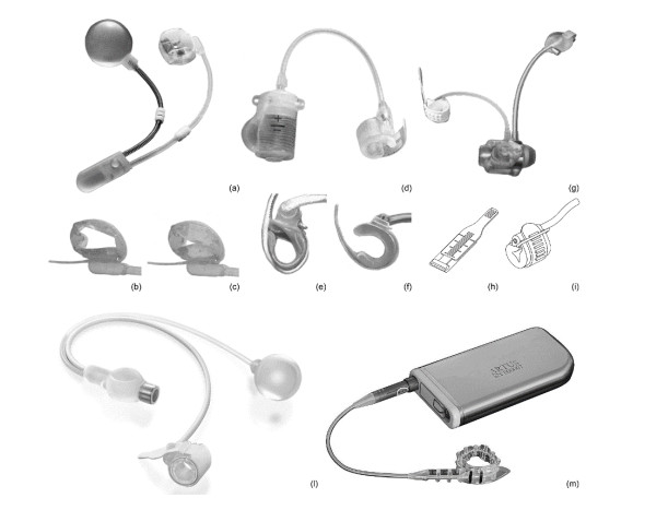
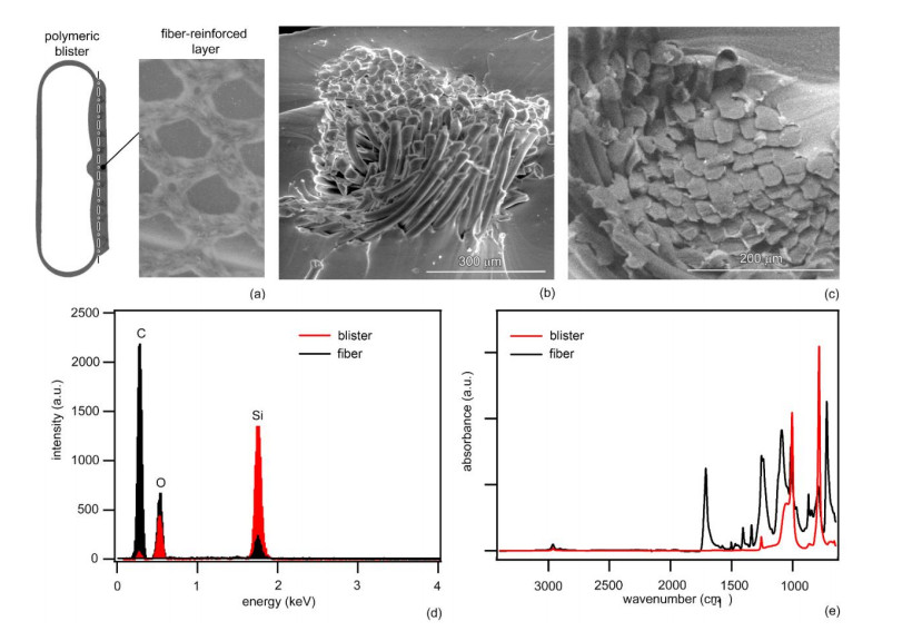
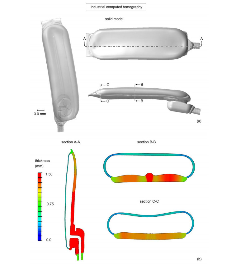
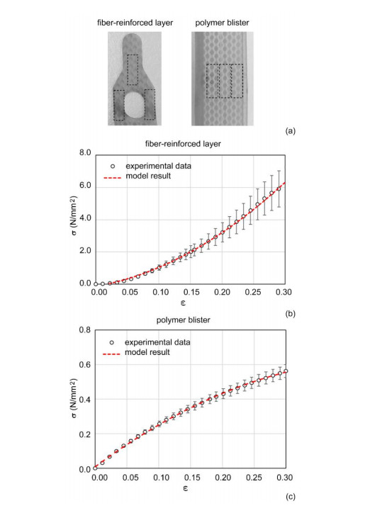
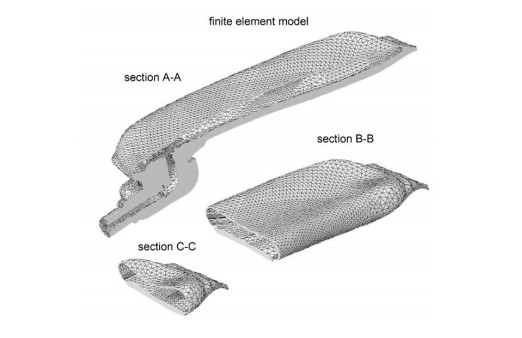
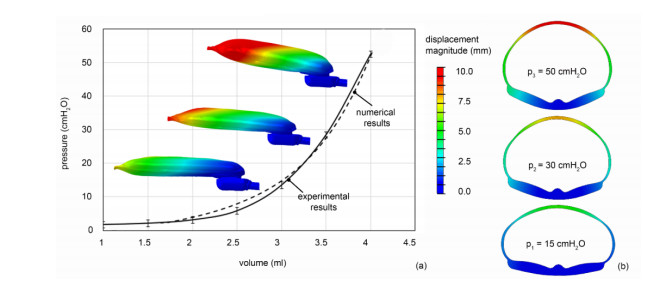
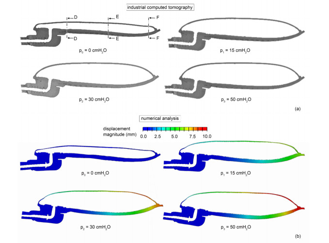
The surgical treatment of urinary incontinence is often performed by adopting an Artificial Urinary Sphincter (AUS). AUS cuff represents a fundamental component of the device, providing the mechanical action addressed to urethral occlusion, which can be investigated by computational approach. In this work, AUS cuff is studied with reference to both materials and structure, to develop a finite element model. Materials behavior is investigated using physicochemical and mechanical characterization, leading to the formulation of a constitutive model. Materials analysis shows that AUS cuff is composed by a silicone blister joined with a PET fiber-reinforced layer. A nonlinear mechanical behavior is found, with a higher stiffness in the outer layer due to fiber-reinforcement. The cuff conformation is acquired by Computer Tomography (CT) both in deflated and inflated conditions, for an accurate definition of the geometrical characteristics. Based on these data, the numerical model of AUS cuff is defined. CT images of the inflated cuff are compared with results of numerical analysis of the inflation process, for model validation. A relative error below 2.5% was found. This study is the first step for the comprehension of AUS mechanical behavior and allows the development of computational tools for the analysis of lumen occlusion process. The proposed approach could be adapted to further fluid-filled cuffs of artificial sphincters.
- artificial urinary sphincter,
- material characterization,
- mechanics characterization,
- micro computed tomography,
- numerical model
Citation: Arturo Nicola Natali, Chiara Giulia Fontanella, Silvia Todros, Piero G. Pavan, Simone Carmignato, Filippo Zanini, Emanuele Luigi Carniel. Conformation and mechanics of the polymeric cuff of artificial urinary sphincter[J]. Mathematical Biosciences and Engineering, 2020, 17(4): 3894-3908. doi: 10.3934/mbe.2020216

Related Papers:

Abstract

The surgical treatment of urinary incontinence is often performed by adopting an Artificial Urinary Sphincter (AUS). AUS cuff represents a fundamental component of the device, providing the mechanical action addressed to urethral occlusion, which can be investigated by computational approach. In this work, AUS cuff is studied with reference to both materials and structure, to develop a finite element model. Materials behavior is investigated using physicochemical and mechanical characterization, leading to the formulation of a constitutive model. Materials analysis shows that AUS cuff is composed by a silicone blister joined with a PET fiber-reinforced layer. A nonlinear mechanical behavior is found, with a higher stiffness in the outer layer due to fiber-reinforcement. The cuff conformation is acquired by Computer Tomography (CT) both in deflated and inflated conditions, for an accurate definition of the geometrical characteristics. Based on these data, the numerical model of AUS cuff is defined. CT images of the inflated cuff are compared with results of numerical analysis of the inflation process, for model validation. A relative error below 2.5% was found. This study is the first step for the comprehension of AUS mechanical behavior and allows the development of computational tools for the analysis of lumen occlusion process. The proposed approach could be adapted to further fluid-filled cuffs of artificial sphincters.

References

[1]	A. D. Markland, P. S. Goode, D. T. Redden, L. G. Borrud, K.L. Burgio, Prevalence of urinary incontinence in men: Results from the national health and nutrition examination survey, J. Urol., 184 (2010), 1022-1027. doi: 10.1016/j.juro.2010.05.025
[2]	I. Milsom, K. S. Coyne, S. Nicholson, M. Kvasz, C. I. Chen, A. J. Wein, Global prevalence and economic burden of urgency urinary incontinence: A systematic review, Eur. Urol., 65 (2014), 79-95. doi: 10.1016/j.eururo.2013.08.031
[3]	B. H. Cordon, N. Singla, A. K. Singla, Artificial urinary sphincters for male stress urinary incontinence: Current perspectives, Med. Devices. (Auckl), 9 (2016), 175-183.
[4]	B. S. Malaeb, S. P, Elliott, J. Lee, D. W. Anderson, G. W. Timm, Novel artificial urinary sphincter in the canine model: The tape mechanical occlusive device, Urology, 77 (2011), 211-216. doi: 10.1016/j.urology.2010.06.065
[5]	C. C. Carson, Artificial urinary sphincter: Current status and future directions, Asian J. Androl., 22 (2020), 154-157. doi: 10.4103/aja.aja_5_20
[6]	P. Weibl, R. Hoelzel, M. Rutkowski, W. Huebner, VICTO and VICTO-plus-novel alternative for the management of postprostatectomy incontinence, early perioperative and postoperative experience, Cent. Eur. J. Urol., 71 (2018), 248-249.
[7]	T. A. Ludwig, P. Reiss, M. Wieland, A. Becker, M. Fisch, F. K. Chun, et al. The ARTUS device: The first feasibility study in human cadavers, Can. J. Urol., 22 (2015), 8100-8104.
[8]	C. A. Hajivassiliou, A review of the complications and results of implantation of the AMS artificial urinary sphincter, Eur. Urol., 35 (1999), 36-44. doi: 10.1159/000019817
[9]	A. C. J. Santos, L.O. Rodrigues, D. C. Azevedo, L. M. Carvalho, M. R. Fernandes, S. O. Avelar, et al., Artificial urinary sphincter for urinary incontinence after radical prostatectomy: A historical cohort from 2004 to 2015, Int. Braz. J. Urol., 43 (2017), 150-154.
[10]	E. Chung, A state-of-the-art review on the evolution of urinary sphincter devices for the treatment of post-prostatectomy urinary incontinence: Past, present and future innovations, J. Med. Eng. Technol., 38 (2014), 328-332.
[11]	A. N. Natali, E. L. Carniel, A. Frigo, P. G. Pavan, S. Todros, P. Pachera, et al., Experimental investigation of the biomechanics of urethral tissues and structures, Exp. Physiol., 101 (2016), 641-656.
[12]	A. N. Natali, E. L. Carniel, C. G. Fontanella, A. Frigo, S. Todros, A. Rubini, et al., Mechanics of the urethral duct: tissue constitutive formulation and structural modeling for the investigation of lumen occlusion, Biomech. Model Mechanobiol., 16 (2017), 439-447.
[13]	F. Marti, T. Leippold, H. John, N. Blunschi, B. Muller, Optimization of the artificial urinary sphincter: modelling and experimental validation, Phys. Med. Biol., 51 (2006), 1361. doi: 10.1088/0031-9155/51/5/023
[14]	A. N. Natali, E. L. Carniel, C. G. Fontanella, Interaction phenomena between a cuff of an artificial urinary sphincter and a urethral phantom, Artif. Organs., 43 (2019), 888-896. doi: 10.1111/aor.13455
[15]	L. De Chiffre, S. Carmignato, J. P. Kruth, R. Schmitt, A. Weckenmann, Industrial applications of computed tomography, CIRP. Ann. Manuf. Techn., 63 (2014), 655-677. doi: 10.1016/j.cirp.2014.05.011
[16]	J. P. Kruth, M. Bartscher, S. Carmignato, R. Schmitt, L. De Chiffre, A. Weckenmann, Computed tomography for dimensional metrology, CIRP Ann. Manuf. Techn., 60 (2011), 821-842. doi: 10.1016/j.cirp.2011.05.006
[17]	M. Sacher G. Schulz, H. Deyle, K. Jager, B. Muller, Comparing the accuracy of intraoral scanners, using advanced micro computed tomography, Proc. SPIE, 11113 (2019), 111131Q.
[18]	B. Müller, Recent trends in high-resolution hard x-ray tomography, Proc. SPIE, 11113 (2019), 1111302.
[19]	J. Von Jackowski, G. Schulz, B. Osmani, T. Tö pper, B. Müller, Three-dimensional characterization of soft silicone elements for intraoral device, Proc. SPIE, 11113 (2019), 1111314.
[20]	C. Vogtlin, G. Schulz, K. Jager, B. Muller, Comparing the accuracy of master models based on digital intra-oral scanners with conventional plaster casts, Phys. Med., 1 (2016), 20-26. doi: 10.1016/j.phmed.2016.04.002
[21]	A. N. Natali, C. G. Fontanella, E. L. Carniel, Biomechanical analysis of the interaction phenomena between artificial urinary sphincter and urethral duct, Int. J. Numer. Meth. Bio., 36 (2020), e3308.
[22]	S. Affatato, F. Zanini, S. Carmignato, Quantification of wear and deformation in different configurations of polyethylene acetabular cups using micro X-ray computed tomography, Materials, 10 (2017), 259. doi: 10.3390/ma10030259
[23]	L. A. Feldkamp, L. C. Davis, J. W. Kress, Practical cone-beam algorithm, J. Opt. Soc. Am. A, 1 (1984), 612-619. doi: 10.1364/JOSAA.1.000612
[24]	S. Carmignato, V. Aloisi, F. Medeossi, F. Zanini, E. Savio, Influence of surface roughness on computed tomography dimensional measurements, CIRP Ann. Manuf. Techn., 66 (2017), 499-502. doi: 10.1016/j.cirp.2017.04.067
[25]	E. L. Carniel, V. Gramigna, C. G. Fontanella, C. Stefanini, A. N. Natali, Constitutive formulation for the mechanical investigation of colonic tissues, J. Biomed. Mat. Res. Part A, 102 (2014), 1243-1254. doi: 10.1002/jbm.a.34787
[26]	A. N. Natali, E. L. Carniel, C. G. Fontanella, S. Todros, G. M. De Benedictis, M. Cerruto, et al., Urethral lumen occlusion by artificial sphincteric devices: A computational biomechanics approach, Biomech. Model Mechanobiol., 16 (2017), 1439-1446.
[27]	E. L. Carniel, A. Frigo, C. G. Fontanella, G. M. De Benedictis, A. Rubini, L. Barp, et al., A biomechanical approach to the analysis of methods and procedures of bariatric surgery, J. Biomech., 56 (2017), 32-41.
[28]	A. N. Natali, E. L. Carniel, A. Frigo, C. G. Fontanella, A. Rubini, Y. Avital, et al., Experimental investigation of the structural behavior of equine urethra, Comput. Methods Programs Biomed., 141 (2017), 35-41.
[29]	Abaqus Documentation, Version 6.14-2, Dassault Systémes Simulia Corp., Providence, RI, 2014. Available from: http://www.130.149.89.49:2080/v6.11/index.html.
[30]	A. N. Natali, C. G. Fontanella, E. L. Carniel, A numerical model for investigating the mechanics of calcaneal fat pad region, J. Mech. Behav. Biomed. Mat., 5 (2012), 216-223. doi: 10.1016/j.jmbbm.2011.08.025
[31]	C. G. Fontanella, E. L. Carniel, A. Forestiero, A. N. Natali, Investigation of the mechanical behaviour of foot skin, Skin Res. Tech., 20 (2014), 445-452. doi: 10.1111/srt.12139
[32]	E. L. Carniel, V. Gramigna, C. G. Fontanella, A. Frigo, C. Stefanini, A. Rubini, et al., Characterization of the anisotropic mechanical behaviour of colon tissues: Experimental activity and constitutive formulation, Exp. Physiol., 99 (2014), 759-771.
[33]	A. N. Natali, A. Audenino, W. Artibani, C.G. Fontanella, E.L. Carniel, E.M. Zanetti, Bladder tissue biomechanical behaviour: Experimental tests and constitutive formulation, J. Biomech., 48 (2015), 3088-3096. doi: 10.1016/j.jbiomech.2015.07.021
[34]	E. A. Romanenko, B. V. Tkachuk, Infrared spectra and structure of thin polydimethylsiloxane films, J. Appl. Spectrosc., 18 (1973), 188-192. doi: 10.1007/BF00604710
[35]	K. Chamerski, M. Lesniak, M. Sitarz, M. Stopa, J. Filipecki, An investigation of the effect of silicone oil on polymer intraocular lenses by means of PALS, FT-IR and Raman spectroscopies, Spectrochim. Acta A, 167 (2016), 96-100.
[36]	L. M. Johnson, L. Gao, I. V. Shields, M. Smith, K. Efimenko, K. Cushing, et al., Elastomeric microparticles for acoustic mediated bioseparations, J. Nanobiotechnol., 28 (2013), 22.
[37]	M. C. Tobin, The infrared spectra of polymers. II. The infrared spectra of polyethylene terephthalate, J. Phys. Chem. US, 61 (1957), 1392-1400.
[38]	C. Y. Liang, S. Krimm, Infrared spectra of high polymers: Part IX. Polyethylene terephthalate, J. Mol. Spectrosc., 3 (1959), 554-574. doi: 10.1016/0022-2852(59)90048-7
[39]	A. A. Ouroumiehei, I. G. Meldrum, Characterization of polyethylene terephthalate and functionalized polypropylene blends by different methods, Iran Polym. J., 8 (1999), 193-204.
[40]	A. N. Natali, C. G. Fontanella, S. Todros, E. L. Carniel, Urethral lumen occlusion by artificial sphincteric device: Evaluation of degraded tissues effects, J. Biomech., 64 (2017), 75-81.
[41]	E. Fattorini, T. Brusa, C. Gingert, S. E. Hieber, V. Leung, B. Osmani, et al., Artificial muscle devices: Innovations ad prospects for fecal incontinence treatment, Annals Biomed. Eng., 44 (2019), 1355-1369.
[42]	A. N. Natali, E. L. Carniel, C. G. Fontanella, Investigation of interaction phenomena between lower urinary tract and artificial urinary sphincter in consideration of urethral tissues degeneration, Biomech. Model Mechanobiol., 2020. Available from: https://link.springer.com/article/10.1007%2Fs10237-020-01326-3.
[43]	E. Ruiz, J. Puigdevall, J. Moldes, P. Lobos, M. Boer, J. Ithurralde, et al., 14 years of experience with the artificial urinary sphincter in children and adolescent without spina bifida, J. Urol., 176 (2006), 1821-1825.
[44]	M. Islah, S. Y. Cho, H. Son, The current role of the artificial urinary sphincter in male and female urinary incontinence, World J. Mens. Health., 31 (2013), 21-30. doi: 10.5534/wjmh.2013.31.1.21

Reader Comments

Your name:*

Email:*
© 2020 the Author(s), licensee AIMS Press. This is an open access article distributed under the terms of the Creative Commons Attribution License (http://creativecommons.org/licenses/by/4.0)