Breast cancer seriously endangers women's life and health, and brings huge economic burden to the family and society. The aim of this study was to analyze the medical expenses and influencing factors of breast cancer patients, and provide theoretical basis for reasonable control of medical expenses of breast cancer patients.
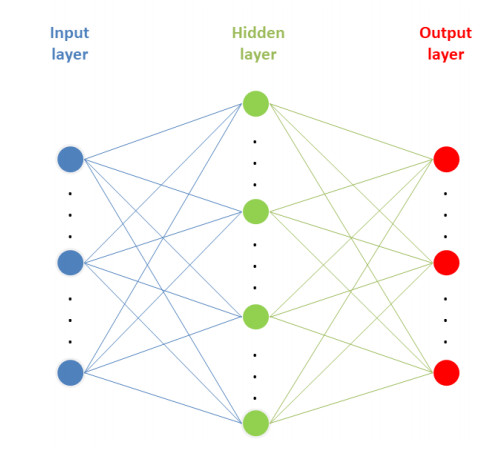
The medical expenses and related information of all female breast cancer patients diagnosed in our hospitals from 2017 to 2019 were collected. Through SSPS Clementine 12.0 software, the back propagation (BP) neural network model and multiple linear regression model were constructed respectively, and the influencing factors of medical expenses of breast cancer patients in the two models were compared.
In the study of medical expenses of breast cancer patients, the prediction error of BP neural network model is less than that of multiple linear regression model. At the same time, the results of the two models showed that the length of stay and region were the top two factors affecting the medical expenses of breast cancer patients.
Compared with multiple linear regression model, BP neural network model is more suitable for the analysis of medical expenses in patients with breast cancer.
Citation: Feiyan Ruan, Xiaotong Ding, Huiping Li, Yixuan Wang, Kemin Ye, Houming Kan. Back propagation neural network model for medical expenses in patients with breast cancer[J]. Mathematical Biosciences and Engineering, 2021, 18(4): 3690-3698. doi: 10.3934/mbe.2021185
Breast cancer seriously endangers women's life and health, and brings huge economic burden to the family and society. The aim of this study was to analyze the medical expenses and influencing factors of breast cancer patients, and provide theoretical basis for reasonable control of medical expenses of breast cancer patients.
The medical expenses and related information of all female breast cancer patients diagnosed in our hospitals from 2017 to 2019 were collected. Through SSPS Clementine 12.0 software, the back propagation (BP) neural network model and multiple linear regression model were constructed respectively, and the influencing factors of medical expenses of breast cancer patients in the two models were compared.
In the study of medical expenses of breast cancer patients, the prediction error of BP neural network model is less than that of multiple linear regression model. At the same time, the results of the two models showed that the length of stay and region were the top two factors affecting the medical expenses of breast cancer patients.
Compared with multiple linear regression model, BP neural network model is more suitable for the analysis of medical expenses in patients with breast cancer.

| [1] |
M. Akram, M. Iqbal, M. Daniyal, A. U. Khan, Awareness and current knowledge of breast cancer, Biol. Res., 50 (2017), 33. doi: 10.1186/s40659-017-0140-9

|
| [2] |
S. Winters, C. Martin, D. Murphy, N. K. Shokar, Breast cancer epidemiology, prevention, and screening, Prog. Mol. Biol. Transl. Sci., 151 (2017), 1-32. doi: 10.1016/bs.pmbts.2017.07.002
|
| [3] |
Z. Anastasiadi, G. D. Lianos, E. Ignatiadou, H. V. Harissis, M. Mitsis, Breast cancer in young women: an overview, Updates Surg., 69 (2017), 313-317. doi: 10.1007/s13304-017-0424-1
|
| [4] |
S. S. Coughlin, Epidemiology of breast cancer in women, Adv. Exp. Med. Biol., 1152 (2019), 9-29. doi: 10.1007/978-3-030-20301-6_2
|
| [5] |
M. A. Thorat, R. Balasubramanian, Breast cancer prevention in high-risk women, Best Pract. Res. Clin. Obstet. Gynaecol., 65 (2020), 18-31. doi: 10.1016/j.bpobgyn.2019.11.006
|
| [6] |
F. Varghese, J. Wong, Breast cancer in the elderly, Surg. Clin. North. Am., 98 (2018), 819-833. doi: 10.1016/j.suc.2018.04.002
|
| [7] |
S. I. Bangdiwala, Regression: multiple linear, Int. J. Inj. Contr. Saf. Promot., 25 (2018), 232-236. doi: 10.1080/17457300.2018.1452336
|
| [8] | Y. H. Hu, S. C. Yu, X. Qi, et al., An overview of multiple linear regression model and its application, Chi. J. Prev. Med., 53 (2019), 653-656. |
| [9] | R. Zemouri, N. Omri, C. Devalland, L. Arnould, B. Morello, N. Zerhouni, et al., Breast cancer diagnosis based on joint variable selection and constructive deep neural network, 2018 IEEE 4th Middle East Conference on Biomedical Engineering (MECBME), 2018. |
| [10] | R. Zemouri, N. Omri, B. Morello, C. Devalland, L. Arnould, N. Zerhouni, et al., Constructive deep neural network for breast cancer diagnosis, IFAC PapersOnLine, 51 (2018), 98-103. |
| [11] | S. Belciug, Artificial Intelligence in Cancer: Diagnostic to Tailored Treatment, Elsevier, New York, 2020. |
| [12] |
Y. Deng, H. Xiao, J. Xu, H. Wang, Prediction model of PSO-BP neural network on coliform amount in special food, Saudi. J. Biol. Sci., 26 (2019), 1154-1160. doi: 10.1016/j.sjbs.2019.06.016
|
| [13] |
Z. Li, Y. Li, A comparative study on the prediction of the BP artificial neural network model and the ARIMA model in the incidence of AIDS, BMC Med. Inf. Decis. Mak., 20 (2020), 143. doi: 10.1186/s12911-020-01157-3
|
| [14] |
X. Liu, Z. Liu, Z. Liang, S. P. Zhu, J. A. F. O. Correia, A. M. P. De Jesus, PSO-BP neural network-based strain prediction of wind turbine blades, Materials, 12 (2019), 1889. doi: 10.3390/ma12121889
|
| [15] | R. Zemouri, N. Omri, F. Fnaiech, N. Zerhouni, N. Fnaiech, A new growing pruning deep learning neural network algorithm (GP-DLNN), Neural Comput. Appl., 32 (2019), 18143-18159. |
| [16] |
J. Li, W. Luo, Hospitalization expenses of acute ischemic stroke patients with atrial fibrillation relative to those with normal sinus rhythm, J. Med. Econ., 20 (2017), 114-120. doi: 10.1080/13696998.2016.1229322
|
| [17] |
M. E. Png, J. Yoong, C. S. Tan, K. S. Chia, Excess hospitalization expenses attributable to type 2 diabetes mellitus in Singapore, Value Health Reg. Issues, 15 (2018), 106-111. doi: 10.1016/j.vhri.2018.02.001
|
| [18] |
J. Wang, P. Li, J. Wen, Impacts of the zero mark-up drug policy on hospitalization expenses of COPD inpatients in Sichuan province, western China: an interrupted time series analysis, BMC Health Serv. Res., 20 (2020), 519. doi: 10.1186/s12913-020-05378-0
|
| [19] | B. Aline, A. M. Zeina, Z. Ryad, S. Valmary-Degano, Prediction of Oncotype DX recurrence score using deep multi-layer perceptrons in estrogen receptor-positive, HER2-negative breast cancer, Breast Cancer, (2020), 1007-1016. |
| [20] |
N. Pandis, Multiple linear regression analysis, Am. J. Orthod. Dentofacial Orthop., 149 (2016), 581. doi: 10.1016/j.ajodo.2016.01.012
|
| [21] | D. G. Streeter, Practical statistics for medical research, New York, Chapman and Hall, 1991. |
| [22] |
G. L. Yuan, L. Z. Liang, Z. F. Zhang, Q. L. Liang, Z. Y. Huang, H. J. Zhang, et al., Hospitalization costs of treating colorectal cancer in China: A retrospective analysis, Medicine, 98 (2019), e16718. doi: 10.1097/MD.0000000000016718
|
| [23] |
X. Zhuang, Y. Chen, Z. Wu, S. R. Scott, M. Zou, Analysis of hospitalization expenses of 610 HIV/AIDS patients in Nantong, China, BMC Health Serv. Res., 20 (2020), 813. doi: 10.1186/s12913-020-05687-4
|
| [24] |
J. Lyu, J. Zhang, BP neural network prediction model for suicide attempt among Chinese rural residents, J. Affect. Disord, 246 (2019), 465-473. doi: 10.1016/j.jad.2018.12.111
|
| [25] |
C. Zhang, R. Zhang, Z. Dai, B. Y. He, Y. Yao, Prediction model for the water jet falling point in fire extinguishing based on a GA-BP neural network, PLoS One, 14 (2019), e0221729. doi: 10.1371/journal.pone.0221729
|
| [26] |
R. Zemouri, N. Zerhouni, D. Racoceanu, Deep learning in the biomedical applications: recent and future status, Appl. Sci., 9 (2019), 1526. doi: 10.3390/app9081526
|
| [27] |
R. Zemouri, C. Devalland, S. Valmary-Degano, N. Zerhounid, Intelligence artificielle: quel avenir en anatomie pathologique?, Ann. de Pathol., 39 (2019), 119-129. doi: 10.1016/j.annpat.2019.01.004
|
Figures(1) / Tables(6)

Feiyan Ruan, Xiaotong Ding, Huiping Li, Yixuan Wang, Kemin Ye, Houming Kan. Back propagation neural network model for medical expenses in patients with breast cancer[J]. Mathematical Biosciences and Engineering, 2021, 18(4): 3690-3698. doi: 10.3934/mbe.2021185


 DownLoad: