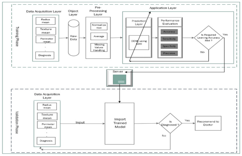
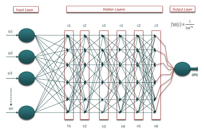
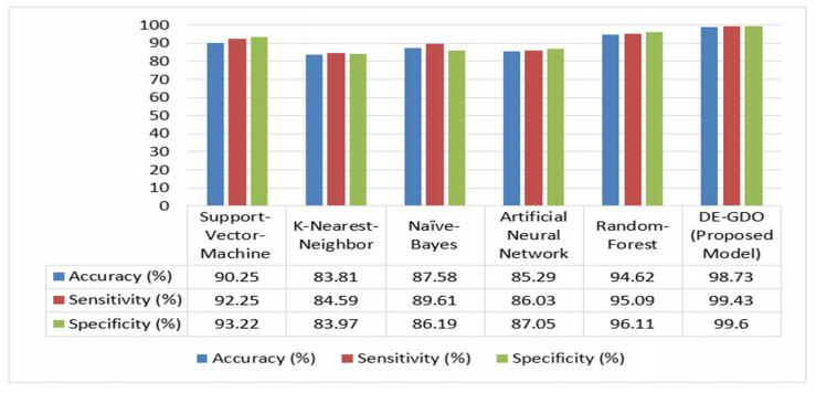
Cancer is a manifestation of disorders caused by the changes in the body's cells that go far beyond healthy development as well as stabilization. Breast cancer is a common disease. According to the stats given by the World Health Organization (WHO), 7.8 million women are diagnosed with breast cancer. Breast cancer is the name of the malignant tumor which is normally developed by the cells in the breast. Machine learning (ML) approaches, on the other hand, provide a variety of probabilistic and statistical ways for intelligent systems to learn from prior experiences to recognize patterns in a dataset that can be used, in the future, for decision making. This endeavor aims to build a deep learning-based model for the prediction of breast cancer with a better accuracy. A novel deep extreme gradient descent optimization (DEGDO) has been developed for the breast cancer detection. The proposed model consists of two stages of training and validation. The training phase, in turn, consists of three major layers data acquisition layer, preprocessing layer, and application layer. The data acquisition layer takes the data and passes it to preprocessing layer. In the preprocessing layer, noise and missing values are converted to the normalized which is then fed to the application layer. In application layer, the model is trained with a deep extreme gradient descent optimization technique. The trained model is stored on the server. In the validation phase, it is imported to process the actual data to diagnose. This study has used Wisconsin Breast Cancer Diagnostic dataset to train and test the model. The results obtained by the proposed model outperform many other approaches by attaining 98.73 % accuracy, 99.60% specificity, 99.43% sensitivity, and 99.48% precision.
Citation: Muhammad Bilal Shoaib Khan, Atta-ur-Rahman, Muhammad Saqib Nawaz, Rashad Ahmed, Muhammad Adnan Khan, Amir Mosavi. Intelligent breast cancer diagnostic system empowered by deep extreme gradient descent optimization[J]. Mathematical Biosciences and Engineering, 2022, 19(8): 7978-8002. doi: 10.3934/mbe.2022373
Cancer is a manifestation of disorders caused by the changes in the body's cells that go far beyond healthy development as well as stabilization. Breast cancer is a common disease. According to the stats given by the World Health Organization (WHO), 7.8 million women are diagnosed with breast cancer. Breast cancer is the name of the malignant tumor which is normally developed by the cells in the breast. Machine learning (ML) approaches, on the other hand, provide a variety of probabilistic and statistical ways for intelligent systems to learn from prior experiences to recognize patterns in a dataset that can be used, in the future, for decision making. This endeavor aims to build a deep learning-based model for the prediction of breast cancer with a better accuracy. A novel deep extreme gradient descent optimization (DEGDO) has been developed for the breast cancer detection. The proposed model consists of two stages of training and validation. The training phase, in turn, consists of three major layers data acquisition layer, preprocessing layer, and application layer. The data acquisition layer takes the data and passes it to preprocessing layer. In the preprocessing layer, noise and missing values are converted to the normalized which is then fed to the application layer. In application layer, the model is trained with a deep extreme gradient descent optimization technique. The trained model is stored on the server. In the validation phase, it is imported to process the actual data to diagnose. This study has used Wisconsin Breast Cancer Diagnostic dataset to train and test the model. The results obtained by the proposed model outperform many other approaches by attaining 98.73 % accuracy, 99.60% specificity, 99.43% sensitivity, and 99.48% precision.

| [1] |
E. Aličković, A. Subasi, Breast cancer diagnosis using GA feature selection and Rotation Forest, Neural Comput. Appl., 28 (2015), 753–763. https://doi.org/10.1007/s00521-015-2103-9 doi: 10.1007/s00521-015-2103-9

|
| [2] | World Health Organization, Breast cancer 2021, 2021. Available from: https://www.who.int/news-room/fact-sheets/detail/breast-cancer. |
| [3] |
Y. S. Sun, Z. Zhao, Z. N. Yang, F. Xu, H. J. Lu, Z. Y. Zhu, et al., Risk factors and preventions of breast cancer, Int. J. Biol. Sci., 13 (2017), 1387–1397. https://doi.org/10.7150/ijbs.21635 doi: 10.7150/ijbs.21635
|
| [4] |
J. B. Harford, Breast-cancer early detection in low-income and middle-income countries: Do what you can versus one size fits all, Lancet Oncol., 12 (2011), 306–312. https://doi.org/10.1016/s1470-2045(10)70273-4 doi: 10.1016/s1470-2045(10)70273-4
|
| [5] |
C. Lerman, M. Daly, C. Sands, A. Balshem, E. Lustbader, T. Heggan, et al., Mammography adherence and psychological distress among women at risk for breast cancer, J. Natl. Cancer Inst., 85 (1993), 1074–1080. https://doi.org/10.1093/jnci/85.13.1074 doi: 10.1093/jnci/85.13.1074
|
| [6] |
P. T. Huynh, A. M. Jarolimek, S. Daye, The false-negative mammogram, Radiographics, 18 (1998), 1137–1154. https://doi.org/10.1148/radiographics.18.5.9747612 doi: 10.1148/radiographics.18.5.9747612
|
| [7] | M. G. Ertosun, D. L. Rubin, Probabilistic Visual Search for Masses within mammography images using Deep Learning, in 2015 IEEE International Conference on Bioinformatics and Biomedicine (BIBM), (2015), 1310–1315. https://doi.org/10.1109/bibm.2015.7359868 |
| [8] | Y. Lu, J. Y. Li, Y. T. Su, A. A. Liu, A review of breast cancer detection in medical images, in 2018 IEEE Visual Communications and Image Processing, (2018), 1–4. https://doi.org/10.1109/vcip.2018.8698732 |
| [9] |
J. Ferlay, I. Soerjomataram, R. Dikshit, S. Eser, C. Mathers, M. Rebelo, et al., Cancer incidence and mortality worldwide: Sources, methods and major patterns in Globocan 2012, Int. J. Cancer, 136 (2014), E359–E386. https://doi.org/10.1002/ijc.29210 doi: 10.1002/ijc.29210
|
| [10] |
N. Mao, P. Yin, Q. Wang, M. Liu, J. Dong, X. Zhang, et al., Added value of Radiomics on mammography for breast cancer diagnosis: A feasibility study, J. Am. Coll. Radiol., 16 (2019), 485–491. https://doi.org/10.1016/j.jacr.2018.09.041 doi: 10.1016/j.jacr.2018.09.041
|
| [11] |
H. Wang, J. Feng, Q. Bu, F. Liu, M. Zhang, Y. Ren, et al., Breast mass detection in digital mammogram based on Gestalt Psychology, J. Healthc. Eng., 2018 (2018), 1–13. https://doi.org/10.1155/2018/4015613 doi: 10.1155/2018/4015613
|
| [12] |
S. McGuire, World cancer report 2014, Switzerland: World Health Organization, international agency for research on cancer, Adv. Nutrit. Int. Rev., 7 (2016), 418–419. https://doi.org/10.3945/an.116.012211 doi: 10.3945/an.116.012211
|
| [13] |
M. K. Gupta, P. Chandra, A comprehensive survey of Data Mining, Int. J. Comput. Technol., 12 (2020), 1243–1257. https://doi.org/10.1007/s41870-020-00427-7 doi: 10.1007/s41870-020-00427-7
|
| [14] | T. Zou, T. Sugihara, Fast identification of a human skeleton-marker model for motion capture system using stochastic gradient descent method, in 2020 8th IEEE RAS/EMBS International Conference for Biomedical Robotics and Biomechatronics (BioRob)., (2020), 181–186. https://doi.org/10.1109/biorob49111.2020.9224442 |
| [15] |
A. Reisizadeh, A. Mokhtari, H. Hassani, R. Pedarsani, An exact quantized decentralized gradient descent algorithm, IEEE Trans. Signal Process., 67 (2019), 4934–4947. https://doi.org/10.1109/tsp.2019.2932876 doi: 10.1109/tsp.2019.2932876
|
| [16] |
D. Maulud, A. M. Abdulazeez, A review on linear regression comprehensive in machine learning, J. Appl. Sci. Technol. Trends, 1 (2020), 140–147. https://doi.org/10.38094/jastt1457 doi: 10.38094/jastt1457
|
| [17] |
D. R. Wilson, T. R. Martinez, The general inefficiency of batch training for gradient descent learning, Neural Networks, 16 (2003) 1429–1451. https://doi.org/10.1016/s0893-6080(03)00138-2 doi: 10.1016/s0893-6080(03)00138-2
|
| [18] |
D. Yi, S. Ji, S. Bu, An enhanced optimization scheme based on gradient descent methods for machine learning, Symmetry, 11 (2019), 942. https://doi.org/10.3390/sym11070942 doi: 10.3390/sym11070942
|
| [19] |
D. A. Zebari, D. Q. Zeebaree, A. M. Abdulazeez, H. Haron, H. N. Hamed, Improved threshold based and trainable fully automated segmentation for breast cancer boundary and pectoral muscle in mammogram images, IEEE Access, 8 (2020), 203097–203116. https://doi.org/10.1109/access.2020.3036072 doi: 10.1109/access.2020.3036072
|
| [20] | D. Q. Zeebaree, H. Haron, A. M. Abdulazeez, D. A. Zebari, Trainable model based on new uniform LBP feature to identify the risk of the breast cancer, in 2019 International Conference on Advanced Science and Engineering (ICOASE), 2019. https://doi.org/10.1109/icoase.2019.8723827 |
| [21] |
D. Q. Zeebaree, A. M. Abdulazeez, L. M. Abdullrhman, D. A. Hasan, O. S. Kareem, The prediction process based on deep recurrent neural networks: A Review, Asian J. Comput. Inf. Syst., 10 (2021), 29–45. https://doi.org/10.9734/ajrcos/2021/v11i230259 doi: 10.9734/ajrcos/2021/v11i230259
|
| [22] |
D. Q. Zeebaree, A. M. Abdulazeez, D. A. Zebari, H. Haron, H. N. A. Hamed, Multi-level fusion in ultrasound for cancer detection based on uniform LBP features, Comput. Matern. Contin., 66 (2021), 3363–3382. https://doi.org/10.32604/cmc.2021.013314 doi: 10.32604/cmc.2021.013314
|
| [23] |
M. Muhammad, D. Zeebaree, A. M. Brifcani, J. Saeed, D. A. Zebari, A review on region of interest segmentation based on clustering techniques for breast cancer ultrasound images, J. Appl. Sci. Technol. Trends, 1 (2020), 78–91. https://doi.org/10.38094/jastt1328 doi: 10.38094/jastt1328
|
| [24] |
P. Kamsing, P. Torteeka, S. Yooyen, An enhanced learning algorithm with a particle filter-based gradient descent optimizer method, Neural Comput. Appl., 32 (2020), 12789–12800. https://doi.org/10.1007/s00521-020-04726-9 doi: 10.1007/s00521-020-04726-9
|
| [25] |
Y. Hamid, L. Journaux, J. A. Lee, M. Sugumaran, A novel method for network intrusion detection based on nonlinear SNE and SVM, J. Artif. Intell. Soft Comput. Res., 6 (2018), 265. https://doi.org/10.1504/ijaisc.2018.097280 doi: 10.1504/ijaisc.2018.097280
|
| [26] | H. Sadeeq, A. M. Abdulazeez, Hardware implementation of firefly optimization algorithm using fpgas, in 2018 International Conference on Advanced Science and Engineering, (2018), 30–35. https://doi.org/10.1109/icoase.2018.8548822 |
| [27] | D. P. Hapsari, I. Utoyo, S. W. Purnami, Fractional gradient descent optimizer for linear classifier support vector machine, in 2020 Third International Conference on Vocational Education and Electrical Engineering (ICVEE), (2020), 1–5. |
| [28] |
M. S. Nawaz, B. Shoaib, M. A. Ashraf, Intelligent cardiovascular disease prediction empowered with gradient descent optimization, Heliyon, 7 (2021), 1–10. https://doi.org/10.1016/j.heliyon.2021.e06948 doi: 10.1016/j.heliyon.2021.e06948
|
| [29] |
Y. Qian, Exploration of machine algorithms based on deep learning model and feature extraction, J. Math. Biosci. Eng., 18 (2021), 7602–7618. https://doi.org/10.3934/mbe.2021376 doi: 10.3934/mbe.2021376
|
| [30] |
Z. Wang, M. Li, H. Wang, H. Jiang, Y. Yao, H. Zhang, et al., Breast cancer detection using extreme learning machine based on feature fusion with CNN deep features, IEEE Access, 7 (2019), 105146–105158. https://doi.org/10.1109/access.2019.2892795 doi: 10.1109/access.2019.2892795
|
| [31] | UCI Machine Learning Repository, Breast Cancer Wisconsin (Diagnostic) Data Set. Available from: https://archive.ics.uci.edu/ml/datasets/Breast+ Cancer + Wisconsin + (Diagnostic). |
| [32] |
R. V. Anji, B. Soni, R. K. Sudheer, Breast cancer detection by leveraging machine learning, ICT Express, 6 (2020), 320–324. https://doi.org/10.1016/j.icte.2020.04.009 doi: 10.1016/j.icte.2020.04.009
|
| [33] |
Z. Salod, Y. Singh, Comparison of the performance of machine learning algorithms in breast cancer screening and detection: A Protocol, J. Public Health Res., 8 (2019). https://doi.org/10.4081/jphr.2019.1677 doi: 10.4081/jphr.2019.1677
|
| [34] |
Y. Lin, H. Luo, D. Wang, H. Guo, K. Zhu, An ensemble model based on machine learning methods and data preprocessing for short-term electric load forecasting, Energies, 10 (2017), 1186. https://doi.org/10.3390/en10081186 doi: 10.3390/en10081186
|
| [35] | M. Amrane, S. Oukid, I. Gagaoua, T. Ensari, Breast cancer classification using machine learning, in 2018 Electric Electronics, Computer Science, Biomedical Engineerings' Meeting (EBBT), (2018), 1–4. https://doi.org/10.1109/ebbt.2018.8391453 |
| [36] |
R. Sumbaly, N. Vishnusri, S. Jeyalatha, Diagnosis of breast cancer using decision tree data mining technique, Int. J. Comput. Appl., 98 (2014), 16–24. https://doi.org/10.5120/17219-7456 doi: 10.5120/17219-7456
|
| [37] |
B. Zheng, S. W. Yoon, S. S. Lam, Breast cancer diagnosis based on feature extraction using a hybrid of k-means and support vector machine algorithms, Expert Syst. Appl., 41 (2014), 1476–1482. https://doi.org/10.1016/j.eswa.2013.08.044 doi: 10.1016/j.eswa.2013.08.044
|
| [38] |
T. Araújo, G. Aresta, E. Castro, J. Rouco, P. Aguiar, C. Eloy, et al., Classification of breast cancer histology images using convolutional neural networks, Plos One, 12 (2017), e0177544. https://doi.org/10.1371/journal.pone.0177544 doi: 10.1371/journal.pone.0177544
|
| [39] | S. P. Rajamohana, A. Dharani, P. Anushree, B. Santhiya, K. Umamaheswari, Machine learning techniques for healthcare applications: early autism detection using ensemble approach and breast cancer prediction using SMO and IBK, in Cognitive Social Mining Applications in Data Analytics and Forensics, (2019), 236–251. https://doi.org/10.4018/978-1-5225-7522-1.ch012 |
| [40] |
L. G. Ahmad, Using three machine learning techniques for predicting breast cancer recurrence, J. Health Med. Inf., 4 (2013), 10–15. https://doi.org/10.4172/2157-7420.1000124 doi: 10.4172/2157-7420.1000124
|
| [41] |
B. Padmapriya, T. Velmurugan, Classification algorithm based analysis of breast cancer data, Int. J. Data Min. Tech. Appl., 5 (2016), 43–49. https://doi.org/10.20894/ijdmta.102.005.001.010 doi: 10.20894/ijdmta.102.005.001.010
|
| [42] | S. Bharati, M. A. Rahman, P. Podder, Breast cancer prediction applying different classification algorithm with comparative analysis using Weka, in 2018 4th International Conference on Electrical Engineering and Information & Communication Technology (ICEEiCT), (2018), 581–584. https://doi.org/10.1109/ceeict.2018.8628084 |
| [43] |
K. Williams, P. A. Idowu, J. A. Balogun, A. I. Oluwaranti, Breast cancer risk prediction using data mining classification techniques, Trans. Networks Commun., 3 (2015), 17–23. https://doi.org/10.14738/tnc.32.662 doi: 10.14738/tnc.32.662
|
| [44] | P. Mekha, N. Teeyasuksaet, Deep learning algorithms for predicting breast cancer based on tumor cells, in 2019 Joint International Conference on Digital Arts, Media and Technology with ECTI Northern Section Conference on Electrical, Electronics, Computer and Telecommunications Engineering (ECTI DAMT-NCON), 2019. https://doi.org/10.1109/ecti-ncon.2019.8692297 |
| [45] | C. Shah, A. G. Jivani, Comparison of data mining classification algorithms for breast cancer prediction, in 2013 Fourth International Conference on Computing, Communications and Networking Technologies (ICCCNT), 2013. https://doi.org/10.1109/icccnt.2013.6726477 |
| [46] |
A. A. Bataineh, A comparative analysis of nonlinear machine learning algorithms for breast cancer detection, Int. J. Mach. Learn. Comput., 9 (2019), 248–254. https://doi.org/10.18178/ijmlc.2019.9.3.794 doi: 10.18178/ijmlc.2019.9.3.794
|
| [47] | M. S. M. Prince, A. Hasan, F. M. Shah, An efficient ensemble method for cancer detection, in 2019 1st International Conference on Advances in Science, Engineering and Robotics Technology (ICASERT), 2019. https://doi.org/10.1109/icasert.2019.8934817 |
| [48] |
S. Aruna, A novel SVM based CSSFFS feature selection algorithm for Detecting Breast Cancer, Int. J. Comput., 31 (2011), 14–20. https://doi.org/10.5120/3844-5346 doi: 10.5120/3844-5346
|
| [49] |
G. Carneiro, J. Nascimento, A. P. Bradley, Automated analysis of unregistered Multi-View Mammograms with deep learning, IEEE Trans. Med. Imaging, 36 (2017), 2355–2365. https://doi.org/10.1109/tmi.2017.2751523 doi: 10.1109/tmi.2017.2751523
|
| [50] |
Z. Sha, L. Hu, B. D. Rouyendegh, Deep learning and optimization algorithms for Automatic Breast Cancer Detection, Int. J. Imaging Syst. Technol., 30 (2020), 495–506. https://doi.org/10.1002/ima.22400 doi: 10.1002/ima.22400
|
| [51] |
M. Mahmoud, Breast cancer classification in histopathological images using convolutional neural network, Int. J. Comput. Sci. Appl., 9 (2018), 12–15. https://doi.org/10.14569/ijacsa.2018.090310 doi: 10.14569/ijacsa.2018.090310
|
| [52] |
Z. Jiao, X. Gao, Y. Wang, J. Li, A deep feature based framework for Breast Masses classification, Neurocomputing, 197 (2016), 221–231. https://doi.org/10.1016/j.neucom.2016.02.060 doi: 10.1016/j.neucom.2016.02.060
|
| [53] |
M. H. Yap, G. Pons, J. Marti, S. Ganau, M. Sentis, R. Zwiggelaar, et al., Automated breast ultrasound lesions detection using convolutional neural networks, IEEE. J. Biomed. Health Inf., 22 (2018), 1218–1226. https://doi.org/10.1109/jbhi.2017.2731873 doi: 10.1109/jbhi.2017.2731873
|
| [54] |
N. Wahab, A. Khan, Y. S. Lee, Transfer learning based deep CNN for segmentation and detection of mitoses in breast cancer histopathological images, Microscopy, 68 (2019), 216–233. https://doi.org/10.1093/jmicro/dfz002 doi: 10.1093/jmicro/dfz002
|
| [55] |
Z. Wang, G. Yu, Y. Kang, Y. Zhao, Q. Qu, Breast tumor detection in digital mammography based on Extreme Learning Machine, Neurocomputing, 128 (2014), 175–184. https://doi.org/10.1016/j.neucom.2013.05.053 doi: 10.1016/j.neucom.2013.05.053
|
| [56] |
Y. Qiu, Y. Wang, S. Yan, M. Tan, S. Cheng, H. Liu, et al., An initial investigation on developing a new method to predict short-term breast cancer risk based on Deep Learning Technology, Comput. Aided. Des., 2016. https://doi.org/10.1117/12.2216275 doi: 10.1117/12.2216275
|
| [57] |
X. W. Chen, X. Lin, Big data deep learning: Challenges and perspectives, IEEE Access, 2 (2014), 514–525. https://doi.org/10.1109/access.2014.2325029 doi: 10.1109/access.2014.2325029
|
| [58] |
J. Arevalo, F. A. González, R. R. Pollán, J. L. Oliveira, M. A. G. Lopez, Representation learning for mammography mass lesion classification with convolutional neural networks, Comput. Methods Programs Biomed., 127 (2016), 248–257. https://doi.org/10.1016/j.cmpb.2015.12.014 doi: 10.1016/j.cmpb.2015.12.014
|
| [59] |
Y. Kumar, A. Aggarwal, S. Tiwari, K. Singh, An efficient and robust approach for biomedical image retrieval using zernike moments, Biomed. Signal Process. Control, 39 (2018), 459–473. https://doi.org/10.1016/j.bspc.2017.08.018 doi: 10.1016/j.bspc.2017.08.018
|
| [60] |
K. Kalaiarasi, R. Soundaria, N. Kausar, P. Agarwal, H. Aydi, H. Alsamir, Optimization of the average monthly cost of an EOQ inventory model for deteriorating items in machine learning using Python, Therm. Sci., 25 (2021), 347–358. https://doi.org/10.2298/tsci21s2347k doi: 10.2298/tsci21s2347k
|
| [61] |
M. Franulović, K. Marković, A. Trajkovski, Calibration of material models for the human cervical spine ligament behaviour using a genetic algorithm, Facta Univ., Series: Mechan. Eng., 19 (2021) 751. https://doi.org/10.22190/fume201029023f doi: 10.22190/fume201029023f
|
| [62] |
M. Fayaz, D. H. Kim, A prediction methodology of energy consumption based on Deep Extreme Learning Machine and comparative analysis in residential buildings, Electronics, 7 (2018), 222. https://doi.org/10.3390/electronics7100222 doi: 10.3390/electronics7100222
|
| [63] |
G. B. Huang, D. H. Wang, Y. Lan, Extreme learning machines: A survey, Int. J. Mach. Learn. Cybern., 2 (2011), 107–122. https://doi.org/10.1007/s13042-011-0019-y doi: 10.1007/s13042-011-0019-y
|
| [64] |
H. Tang, S. Gao, L. Wang, X. Li, B. Li, S. Pang, A novel intelligent fault diagnosis method for rolling bearings based on Wasserstein generative adversarial network and Convolutional Neural Network under Unbalanced Dataset, Sensors, 21 (2021), 6754. https://doi.org/10.3390/s21206754 doi: 10.3390/s21206754
|
| [65] |
J. Wei, H. Liu, G. Yan, F. Sun, Multi-modal deep extreme learning machine for robotic grasping recognition, Proceed. Adapt., Learn. Optim., (2016), 223–233. https://doi.org/10.1007/978-3-319-28373-9_19 doi: 10.1007/978-3-319-28373-9_19
|
| [66] |
N. S. Naz, M. A. Khan, S. Abbas, A. Ather, S. Saqib, Intelligent routing between capsules empowered with deep extreme machine learning technique, SN Appl. Sci., 2 (2019), 1–14. https://doi.org/10.1007/s42452-019-1873-6 doi: 10.1007/s42452-019-1873-6
|
| [67] |
J. Cai, J. Luo, S. Wang, S. Yang, Feature selection in Machine Learning: A new perspective, Neurocomputing, 300 (2018), 70–79. https://doi.org/10.1016/j.neucom.2017.11.077 doi: 10.1016/j.neucom.2017.11.077
|
| [68] |
L. M. Abualigah, A. T. Khader, E. S. Hanandeh, A new feature selection method to improve the document clustering using particle swarm optimization algorithm, J. Comput. Sci., 25 (2018), 456–466. https://doi.org/10.1016/j.jocs.2017.07.018 doi: 10.1016/j.jocs.2017.07.018
|
| [69] |
P. A. Flach, ROC analysis, encyclopedia of machine learning and data mining, Encycl. Mach. Learn. Data Min., (2016), 1–8. https://doi.org/10.1007/978-1-4899-7502-7_739-1 doi: 10.1007/978-1-4899-7502-7_739-1
|
| [70] |
Q. Wuniri, W. Huangfu, Y. Liu, X. Lin, L. Liu, Z. Yu, A generic-driven wrapper embedded with feature-type-aware hybrid bayesian classifier for breast cancer classification, IEEE Access, 7 (2019), 119931–119942. https://doi.org/10.1109/access.2019.2932505 doi: 10.1109/access.2019.2932505
|
| [71] |
J. Zheng, D. Lin, Z. Gao, S. Wang, M. He, J. Fan, Deep Learning assisted efficient ADABOOST algorithm for breast cancer detection and early diagnosis, IEEE Access, 8 (2020), 96946–96954. https://doi.org/10.1109/access.2020.2993536 doi: 10.1109/access.2020.2993536
|
| [72] |
X. Zhang, D. He, Y. Zheng, H. Huo, S. Li, R. Chai, et al., Deep learning based analysis of breast cancer using advanced ensemble classifier and linear discriminant analysis, IEEE Access, 8 (2020), 120208–120217. https://doi.org/10.1109/access.2020.3005228 doi: 10.1109/access.2020.3005228
|
| [73] |
Y. Yari, T. V. Nguyen, H. T. Nguyen, Deep learning applied for histological diagnosis of breast cancer, IEEE Access, 8 (2020), 162432–162448. https://doi.org/10.1109/access.2020.3021557 doi: 10.1109/access.2020.3021557
|
| [74] |
A. H. Osman, H. M. Aljahdali, An effective of ensemble boosting learning method for breast cancer virtual screening using neural network model, IEEE Access, 8 (2020), 39165–39174. https://doi.org/10.1109/access.2020.2976149 doi: 10.1109/access.2020.2976149
|
| [75] |
Y. Li, J. Wu, Q. Wu, Classification of breast cancer histology images using multi-size and discriminative patches based on Deep Learning, IEEE Access, 7 (2019), 21400–21408. https://doi.org/10.1109/access.2019.2898044 doi: 10.1109/access.2019.2898044
|
| [76] |
D. M. Vo, N. Q. Nguyen, S. W. Lee, Classification of breast cancer histology images using incremental boosting convolution networks, Inf. Sci., 482 (2019), 123–138. https://doi.org/10.1016/j.ins.2018.12.089 doi: 10.1016/j.ins.2018.12.089
|
| [77] |
S. Y. Siddiqui, M. A. Khan, S. Abbas, F. Khan, Smart occupancy detection for road traffic parking using deep extreme learning machine, J. K.S.U. Comput. Inf. Sci., 34 (2022), 727–733. https://doi.org/10.1016/j.jksuci.2020.01.016 doi: 10.1016/j.jksuci.2020.01.016
|
| [78] |
M. A. Khan, S. Abbas, K. M. Khan, M. A. A. Ghamdi, A. Rehman, Intelligent forecasting model of covid-19 novel coronavirus outbreak empowered with deep extreme learning machine, Comput. Matern. Contin., 64 (2020), 1329–1342. https://doi.org/10.32604/cmc.2020.011155 doi: 10.32604/cmc.2020.011155
|
| [79] |
S. Abbas, M. A. Khan, L. E. F. Morales, A. Rehman, Y. Saeed, Modelling, simulation and optimization of power plant energy sustainability for IoT enabled smart cities empowered with deep extreme learning machine, IEEE Access, 8 (2020), 39982–39997. https://doi.org/10.1109/ACCESS.2020.2976452 doi: 10.1109/ACCESS.2020.2976452
|
| [80] |
A. Rehman, A. Athar, M. A. Khan, S. Abbas, A. Fatima, M. Zareei, et al., Modelling, simulation, and optimization of diabetes type ii prediction using deep extreme learning machine, J. Ambient Intell. Smart Environ., 12 (2020), 125–138. https://doi.org/10.3233/AIS-200554 doi: 10.3233/AIS-200554
|
| [81] |
A. Haider, M. A. Khan, A. Rehman, H. S. Kim, A real-time sequential deep extreme learning machine cybersecurity intrusion detection system, Comput. Matern. Contin., 66 (2021), 1785–1798. https://doi.org/10.32604/cmc.2020.013910 doi: 10.32604/cmc.2020.013910
|
| [82] |
M. A. Khan, A. Rehman, K. M. Khan, M. A. A. Ghamdi, S. H. Almotiri, Enhance intrusion detection in computer networks based on deep extreme learning machine, Comput. Matern. Contin., 66 (2021), 467–480. https://doi.org/10.32604/cmc.2020.013121 doi: 10.32604/cmc.2020.013121
|
| [83] |
U. Ahmed, G. F. Issa, M. A. Khan, S. Aftab, M. F. Khan, R. A. T. Said, et al., Prediction of diabetes empowered with fused machine learning, IEEE Access, 10 (2022), 8529–8538. https://doi.org/10.1109/ACCESS.2022.3142097 doi: 10.1109/ACCESS.2022.3142097
|
| [84] |
S. Y. Siddiqui, A. Haider, T. M. Ghazal, M. A. Khan, I. Naseer, S. Abbas, et al., IoMT cloud-based intelligent prediction of breast cancer stages empowered with deep learning, IEEE Access, 9 (2021), 146478–146491. https://doi.org/10.1109/ACCESS.2021.3123472 doi: 10.1109/ACCESS.2021.3123472
|
| [85] |
M. Ahmad, M. Alfayad, S. Aftab, M. A. Khan, A. Fatima, B. Shoaib, et.al., Data and machine learning fusion architecture for cardiovascular disease prediction, Comput. Matern. Contin., 69 (2021), 2717–2731. https://doi.org/10.32604/cmc.2021.019013 doi: 10.32604/cmc.2021.019013
|
Figures(4) / Tables(4)

Muhammad Bilal Shoaib Khan, Atta-ur-Rahman, Muhammad Saqib Nawaz, Rashad Ahmed, Muhammad Adnan Khan, Amir Mosavi. Intelligent breast cancer diagnostic system empowered by deep extreme gradient descent optimization[J]. Mathematical Biosciences and Engineering, 2022, 19(8): 7978-8002. doi: 10.3934/mbe.2022373


 DownLoad: