Powerlifting score prediction using a machine learning method

Vinh Huy Chau; Vinh Huy Chau

doi:10.3934/mbe.2021056

Mathematical Biosciences and Engineering

2021, Volume 18, Issue 2: 1040-1050. doi: 10.3934/mbe.2021056

Previous Article Next Article

Research article Special Issues

Powerlifting score prediction using a machine learning method

Vinh Huy Chau ^,

Ho Chi Minh City University of Physical Education and Sport, Ho Chi Minh City 700000, Vietnam

Received: 03 December 2020 Accepted: 30 December 2020 Published: 07 January 2021

This research discusses an interesting topic, using artificial intelligence methods to predict the score of powerlifters. We collected the characteristics of powerlifters, and then used the reservoir computing extreme learning machine to build a predictive model. In order to further improve the prediction results, we propose a method to optimize the reservoir computing extreme learning machine using the whale optimization algorithm. Experimental results show that our proposed method can effectively predict the score of powerlifters with the coefficient of determination value is 0.7958 and root-mean-square error of prediction value is 16.73. This provides a reliable basis for experts to judge the results before the competition.
- artificial intelligence,
- machine learning,
- powerlifting,
- score prediction
Citation: Vinh Huy Chau. Powerlifting score prediction using a machine learning method[J]. Mathematical Biosciences and Engineering, 2021, 18(2): 1040-1050. doi: 10.3934/mbe.2021056

Related Papers:

Abstract

This research discusses an interesting topic, using artificial intelligence methods to predict the score of powerlifters. We collected the characteristics of powerlifters, and then used the reservoir computing extreme learning machine to build a predictive model. In order to further improve the prediction results, we propose a method to optimize the reservoir computing extreme learning machine using the whale optimization algorithm. Experimental results show that our proposed method can effectively predict the score of powerlifters with the coefficient of determination value is 0.7958 and root-mean-square error of prediction value is 16.73. This provides a reliable basis for experts to judge the results before the competition.

References

[1]	D. J. V. D. Windt, V. Sud, H. Zhang, A. Tsung, H. Huang, The effects of physical exercise on fatty liver disease, J. Liver Res., 18 (2018), 89–101.
[2]	D. Song, D. S. F. Yu, P. W. C. Li, Y. Lei, The effectiveness of physical exercise on cognitive and psychological outcomes in individuals with mild cognitive impairment: A systematic review and meta-analysis, Int. J. Nurs. Stud., 79 (2018), 155–164. doi: 10.1016/j.ijnurstu.2018.01.002
[3]	M. G. Benedetti, G. Furlini, A. Zati, G. L. Mauro, The effectiveness of physical exercise on bone density in osteoporotic patients, Bio. Med. Res. Int., (2018), 4840531.
[4]	M. M. Ziaaldini, E. Marzetti, A. Picca, Z. Murlasits, Biochemical pathways of sarcopenia and their modulation by physical exercise: A narrative review, Front. Med., 4 (2017), 167. doi: 10.3389/fmed.2017.00167
[5]	C. M. Hearing, W. C. Chang, K. L. Szuhany, T. Deckersbach, A. A. Nierenberg, L. G. Sylvia, Physical exercise for treatment of mood disorders: A critical review, Curr. Behav. Neurosci. Rep., 3 (2016), 350–359. doi: 10.1007/s40473-016-0089-y
[6]	L. W. Judge, L. J. Urbina, D. L. Hoover, B. W. Craig, L. M. Judge, B. M. Leitzelar, et al., The impact of competitive trait anxiety on collegiate powerlifting performance, J. Strength Cond. Res., 30 (2016), 2399–2405.
[7]	M. Mottaghi, A. Atarodi, Z. Rohani, The relationship between coaches' and athletes' competitive anxiety and their performance, Iran. J. Psychiatry Behav. Sci., 7 (2013), 68–76.
[8]	H. J. Pritchard, D. A. Tod, M. J. Barnes, J. W. Keogh, M. R. McGuigan, Tapering practices of New Zealand's elite raw powerlifters, J. Strength Cond. Res., 30 (2016), 1796–1804. doi: 10.1519/JSC.0000000000001292
[9]	M. Zawadka, M. S. Paszkowska, P. Gawda, E. Lukasik, J. Smolka, M. Jablonski, What factors can affect lumbopelvic flexion-extension motion in the sagittal plane?: A literature review, Hum. Mov. Sci., 58 (2018), 205–218. doi: 10.1016/j.humov.2018.02.008
[10]	A. C. Fry, W. J. Kraemer, M. H. Stone, L. P. Koziris, J. T. Thrush, S. J. Fleck, Relationships between serum testosterone, cortisol and weightlifting performance, J. Strength Cond. Res., 14 (2000), 338–343.
[11]	I. Sandau, M. Witt, The influence of stress factors on joint loading of lower extremities in weightlifting, Ger. J. Sports Med./Deutsch. Z. Sportmed., 69 (2018), 1–10.
[12]	P. A. Solberg, W. G. Hopkins, G. Paulsen, T. A. Haugen, Peak age and performance progression in world-class weightlifting and powerlifting athletes, Int. J. Sports Physiol. Perform., (2019), 1–24.
[13]	C. Latella, W. P. Teo, J. Spathis, D. V. D. Hoek, Long-term strength adaptation: A 15-year analysis of powerlifting athletes, J. Strength Cond. Res., 34 (2020), 2412. doi: 10.1519/JSC.0000000000003657
[14]	C. Latella, D. V. D. Hoek, W. P. Teo, Factors affecting powerlifting performance: an analysis of age-and weight-based determinants of relative strength, Int. J. Perform. Anal. Sport, 18 (2018), 532–544. doi: 10.1080/24748668.2018.1496393
[15]	M. M. Anton, W. W. Spirduso, H. Tanaka, Age-related declines in anaerobic muscular performance: Weightlifting and powerlifting, Med. Sci. Sports Exercise, 36 (2014), 143–147.
[16]	L. P. James, P. Comfort, T. J. Suchomel, V. G. Kelly, E. M. Beckman, G. G. Haff, The impact of power clean ability and training age on adaptations to weightlifting-style training, J. Strength Cond. Res., 33 (2019), 2936–2944. doi: 10.1519/JSC.0000000000002534
[17]	J. Pearson, J. G. Spathis, D. J. V. D. Hoek, P. J. Owen, J. Weakley, C. Latella, Effect of competition frequency on strength performance of powerlifting athletes, J. Strength Cond. Res., 34 (2020), 1213–1219. doi: 10.1519/JSC.0000000000003563
[18]	N. A. Coker, A. N. Varanoske, K. M. Baker, D. L. H. Vaughn, A. J. Wells, Predictors of competitive success of national-level powerlifters: A multilevel analysis, Int. J. Perform. Anal. Sport, 18 (2018), 796–805. doi: 10.1080/24748668.2018.1519751
[19]	S. K. Travis, M. C. Zourdos, C. D. Bazyler, Weight selection attempts of elite classic powerlifters, Percept. Mot. Skills, 2020.
[20]	M. Z. Naser, A. Alavi, Insights into performance fitness and error metrics for machine learning, preprint, arXiv: 2006.00887.
[21]	A. Botchkarev, Performance metrics (error measures) in machine learning regression, forecasting and prognostics: Properties and typology, preprint, arXiv: 1809.03006.
[22]	G. B. Huang, Q. Y. Zhu, C. K. Siew, Extreme learning machine: Theory and applications, Neurocomputing, 70 (2006), 489–501. doi: 10.1016/j.neucom.2005.12.126
[23]	M. Rocca, C. Perna, Nonlinear autoregressive sieve bootstrap based on extreme learning machines, Math. Biosci. Eng., 17 (2019), 636–653.
[24]	G. B. Huang, H. Zhou, X. Ding, R. Zhang, Extreme learning machine for regression and multiclass classification, IEEE Trans. Syst., Man, Cybern., Part B (Cybern.), 42 (2011), 513–529.
[25]	J. Tang, C. Deng, G. B. Huang, Extreme learning machine for multilayer perceptron, IEEE Trans. Neural Networks Learn. Syst., 27 (2015), 809–821.
[26]	W. Deng, Q. Zheng, L. Chen, Regularized extreme learning machine, 2009 IEEE Symp. Comput. Intel. Data Min., (2009), 389–395.
[27]	Y. Zheng, B. Chen, S. Wang, W. Wang, W. Qin, Mixture correntropy-based kernel extreme learning machines, IEEE Trans. Neural Networks Learn. Syst., 2020.
[28]	J. Cao, H. Dai, B. Lei, C. Yin, H. Zeng, A. Kummert, Maximum correntropy criterion-based hierarchical one-class classification, IEEE Trans. Neural Networks Learn. Syst., 2020.
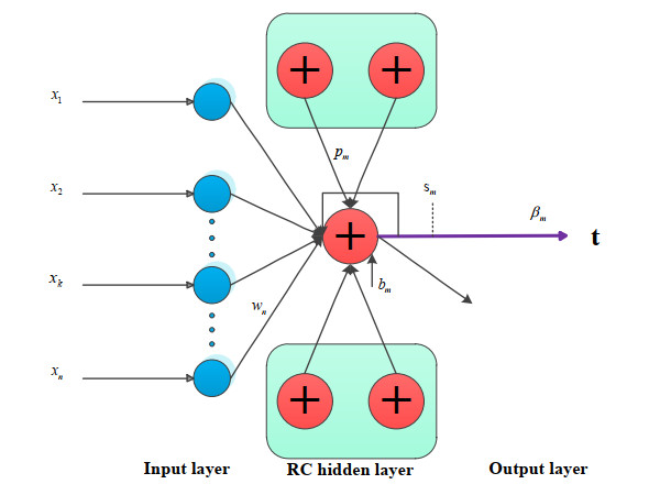
[29]	O. F. Ertugrul, A novel randomized machine learning approach: Reservoir computing extreme learning machine. Appl. Soft Comput., 94 (2020), 106433. doi: 10.1016/j.asoc.2020.106433
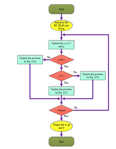
[30]	S. Mirjalili, A. Lewis, The whale optimization algorithm. Adv. Eng. Software, 95 (2016), 51–67. doi: 10.1016/j.advengsoft.2016.01.008
[31]	L. L. Li, J. Sun, M. L. Tseng, Z. G. Li, Extreme learning machine optimized by whale optimization algorithm using insulated gate bipolar transistor module aging degree evaluation, Expert Syst. Appl., 127 (2019), 58–67. doi: 10.1016/j.eswa.2019.03.002
[32]	https://www.powerlifting.sport/championships/results.html
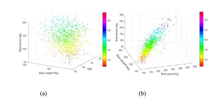
[33]	https://www.kaggle.com/open-powerlifting/powerlifting-database
[34]	T. Yang, Study on the growth rule of the olympic men's weightlifting champion and winning factors. Sichuan Sports Sci., 38 (2019), 54–58.
[35]	B. T. Le, D. Xiao, Y. Mao, D. He, Coal analysis based on visible-infrared spectroscopy and a deep neural network, Infrared Phys. Technol., 93 (2018), 34–40. doi: 10.1016/j.infrared.2018.07.013
[36]	D. Xiao, B. T. Le, Rapid analysis of coal characteristics based on deep learning and visible-infrared spectroscopy, Microchem. J., (2020), 104880.

Reader Comments

Your name:*

Email:*
© 2021 the Author(s), licensee AIMS Press. This is an open access article distributed under the terms of the Creative Commons Attribution License (http://creativecommons.org/licenses/by/4.0)