Synchronization of Clifford-valued neural networks with leakage, time-varying, and infinite distributed delays on time scales

Călin-Adrian Popa; Călin-Adrian Popa

doi:10.3934/math.2024915

AIMS Mathematics

2024, Volume 9, Issue 7: 18796-18823. doi: 10.3934/math.2024915

Previous Article Next Article

Research article

Synchronization of Clifford-valued neural networks with leakage, time-varying, and infinite distributed delays on time scales

Călin-Adrian Popa ^,

Department of Computers and Information Technology, Politehnica University of Timişoara, Blvd. V. Pârvan, No. 2, 300223 Timişoara, Romania

Received: 08 February 2024 Revised: 22 April 2024 Accepted: 06 May 2024 Published: 04 June 2024
MSC : 93C10, 93C43, 93D23

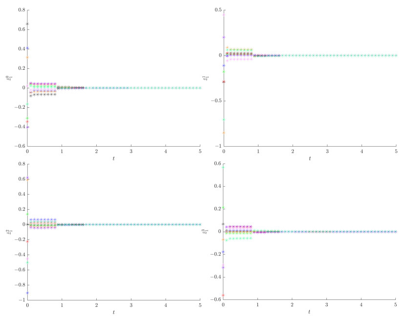
Neural networks (NNs) with values in multidimensional domains have lately attracted the attention of researchers. Thus, complex-valued neural networks (CVNNs), quaternion-valued neural networks (QVNNs), and their generalization, Clifford-valued neural networks (ClVNNs) have been proposed in the last few years, and different dynamic properties were studied for them. On the other hand, time scale calculus has been proposed in order to jointly study the properties of continuous time and discrete time systems, or any hybrid combination between the two, and was also successfully applied to the domain of NNs. Finally, in real implementations of NNs, time delays occur inevitably. Taking all these facts into account, this paper discusses ClVNNs defined on time scales with leakage, time-varying delays, and infinite distributed delays, a type of delays which have been relatively rarely present in the existing literature. A state feedback control scheme and a generalization of the Halanay inequality for time scales are used in order to obtain sufficient conditions expressed as algebraic inequalities and as linear matrix inequalities (LMIs), using two general Lyapunov-like functions, for the exponential synchronization of the proposed model. Two numerical examples are given in order to illustrate the theoretical results.
- Clifford-valued neural networks (ClVNNs),
- synchronization analysis,
- time scales,
- time delays,
- infinite distributed delays
Citation: Călin-Adrian Popa. Synchronization of Clifford-valued neural networks with leakage, time-varying, and infinite distributed delays on time scales[J]. AIMS Mathematics, 2024, 9(7): 18796-18823. doi: 10.3934/math.2024915

Related Papers:

Abstract

Neural networks (NNs) with values in multidimensional domains have lately attracted the attention of researchers. Thus, complex-valued neural networks (CVNNs), quaternion-valued neural networks (QVNNs), and their generalization, Clifford-valued neural networks (ClVNNs) have been proposed in the last few years, and different dynamic properties were studied for them. On the other hand, time scale calculus has been proposed in order to jointly study the properties of continuous time and discrete time systems, or any hybrid combination between the two, and was also successfully applied to the domain of NNs. Finally, in real implementations of NNs, time delays occur inevitably. Taking all these facts into account, this paper discusses ClVNNs defined on time scales with leakage, time-varying delays, and infinite distributed delays, a type of delays which have been relatively rarely present in the existing literature. A state feedback control scheme and a generalization of the Halanay inequality for time scales are used in order to obtain sufficient conditions expressed as algebraic inequalities and as linear matrix inequalities (LMIs), using two general Lyapunov-like functions, for the exponential synchronization of the proposed model. Two numerical examples are given in order to illustrate the theoretical results.

References

[1]	J. K. Pearson, D. L. Bisset, Neural networks in the Clifford domain, In Proceedings of 1994 IEEE International Conference on Neural Networks (ICNN'94), IEEE, 1994. https://doi.org/10.1109/icnn.1994.374502
[2]	J. R. Vallejo, E. Bayro-Corrochano, Clifford Hopfield Neural Networks, In 2008 IEEE International Joint Conference on Neural Networks (IEEE World Congress on Computational Intelligence), IEEE, 2008. https://doi.org/10.1109/ijcnn.2008.4634314
[3]	Y. Liu, P. Xu, J. Lu, J. Liang, Global stability of Clifford-valued recurrent neural networks with time delays, Nonlinear Dyn., 84 (2015), 767–777. https://doi.org/10.1007/s11071-015-2526-y doi: 10.1007/s11071-015-2526-y
[4]	Y. Li, J. Xiang, Existence and global exponential stability of anti-periodic solution for Clifford-valued inertial Cohen–Grossberg neural networks with delays, Neurocomputing, 332 (2019), 259–269. https://doi.org/10.1016/j.neucom.2018.12.064 doi: 10.1016/j.neucom.2018.12.064
[5]	B. Li, Y. Li, Existence and Global Exponential Stability of Almost Automorphic Solution for Clifford-Valued High-Order Hopfield Neural Networks with Leakage Delays, Complexity, 2019 (2019), 6751806. https://doi.org/10.1155/2019/6751806 doi: 10.1155/2019/6751806
[6]	B. Li, Y. Li, Existence and Global Exponential Stability of Pseudo Almost Periodic Solution for Clifford- Valued Neutral High-Order Hopfield Neural Networks With Leakage Delays, IEEE Access, 7 (2019), 150213–150225. https://doi.org/10.1109/access.2019.2947647 doi: 10.1109/access.2019.2947647
[7]	G. Rajchakit, R. Sriraman, P. Vignesh, C.P. Lim, Impulsive effects on Clifford-valued neural networks with time-varying delays: An asymptotic stability analysis, Appl. Math. Comput., 407 (2021), 126309. https://doi.org/10.1016/j.amc.2021.126309 doi: 10.1016/j.amc.2021.126309
[8]	G. Rajchakit, R. Sriraman, N. Boonsatit, P. Hammachukiattikul, C. P. Lim, P. Agarwal, Exponential stability in the Lagrange sense for Clifford-valued recurrent neural networks with time delays, Adv. Differ. Equations, 2021 (2021), 256. https://doi.org/10.1186/s13662-021-03415-8 doi: 10.1186/s13662-021-03415-8
[9]	G. Rajchakit, R. Sriraman, N. Boonsatit, P. Hammachukiattikul, C. P. Lim, P. Agarwal, Global exponential stability of Clifford-valued neural networks with time-varying delays and impulsive effects, Adv. Differ. Equations, 2021 (2021), 208. https://doi.org/10.1186/s13662-021-03367-z doi: 10.1186/s13662-021-03367-z
[10]	N. Huo, B. Li, Y. Li, Global exponential stability and existence of almost periodic solutions in distribution for Clifford-valued stochastic high-order Hopfield neural networks with time-varying delays, AIMS Math., 7 (2022), 3653–3679. https://doi.org/10.3934/math.2022202 doi: 10.3934/math.2022202
[11]	G. Rajchakit, R. Sriraman, C. P. Lim, B. Unyong, Existence, uniqueness and global stability of Clifford-valued neutral-type neural networks with time delays, Math. Comput. Simul., 201 (2022), 508–527. https://doi.org/10.1016/j.matcom.2021.02.023 doi: 10.1016/j.matcom.2021.02.023
[12]	R. Sriraman, A. Nedunchezhiyan, Global stability of Clifford-valued Takagi-Sugeno fuzzy neural networks with time-varying delays and impulses, Kybernetika, 58 (2022), 498–521. https://doi.org/10.14736/kyb-2022-4-0498 doi: 10.14736/kyb-2022-4-0498
[13]	A. M. Alanazi, R. Sriraman, R. Gurusamy, S. Athithan, P. Vignesh, Z. Bassfar, et al., System decomposition method-based global stability criteria for T-S fuzzy Clifford-valued delayed neural networks with impulses and leakage term, AIMS Math., 8 (2023), 15166–15188. https://doi.org/10.3934/math.2023774 doi: 10.3934/math.2023774
[14]	E. A. Assali, A spectral radius-based global exponential stability for Clifford-valued recurrent neural networks involving time-varying delays and distributed delays, Comput. Appl. Math., 42 (2023), 48. https://doi.org/10.1007/s40314-023-02188-y doi: 10.1007/s40314-023-02188-y
[15]	Y. Li, S. Shen, Pseudo almost periodic synchronization of Clifford-valued fuzzy cellular neural networks with time-varying delays on time scales, Adv. Differ. Equations, 2020 (2020), 593. https://doi.org/10.1186/s13662-020-03041-w doi: 10.1186/s13662-020-03041-w
[16]	J. Gao, X. Huang, L. Dai, Weighted Pseudo Almost Periodic Synchronization for Clifford-Valued Neural Networks with Leakage Delay and Proportional Delay, Acta Appl. Math., 186 (2023), 11. https://doi.org/10.1007/s10440-023-00587-1 doi: 10.1007/s10440-023-00587-1
[17]	G. Rajchakit, R. Sriraman, C. P. Lim, P. Sam-ang, P. Hammachukiattikul, Synchronization in Finite-Time Analysis of Clifford-Valued Neural Networks with Finite-Time Distributed Delays, Mathematics, 9 (2021), 1163. https://doi.org/10.3390/math9111163 doi: 10.3390/math9111163
[18]	N. Boonsatit, R. Sriraman, T. Rojsiraphisal, C. P. Lim, P. Hammachukiattikul, G. Rajchakit, Finite-Time Synchronization of Clifford-Valued Neural Networks With Infinite Distributed Delays and Impulses, IEEE Access, 9 (2021), 111050–111061. https://doi.org/10.1109/access.2021.3102585 doi: 10.1109/access.2021.3102585
[19]	N. Boonsatit, G. Rajchakit, R. Sriraman, C. P. Lim, P. Agarwal, Finite-/fixed-time synchronization of delayed Clifford-valued recurrent neural networks, Adv. Differ. Equations, 2021 (2021), 276. https://doi.org/10.1186/s13662-021-03438-1 doi: 10.1186/s13662-021-03438-1
[20]	C. Aouiti, F. Touati, Global dissipativity of Clifford-valued multidirectional associative memory neural networks with mixed delays, Comput. Appl. Math., 39 (2020), 310. https://doi.org/10.1007/s40314-020-01367-5 doi: 10.1007/s40314-020-01367-5
[21]	J. Wang, X. Wang, X. Zhang, S. Zhu, Global h-Synchronization for High-Order Delayed Inertial Neural Networks via Direct SORS Strategy, IEEE Trans. Syst. Man Cybern.: Syst., 53 (2023), 6693–6704. https://doi.org/10.1109/tsmc.2023.3286095 doi: 10.1109/tsmc.2023.3286095
[22]	Q. Li, H. Wei, D. Hua, J. Wang, J. Yang, Stabilization of Semi-Markovian Jumping Uncertain Complex-Valued Networks with Time-Varying Delay: A Sliding-Mode Control Approach, Neural Process. Lett., 56 (2024), 111. https://doi.org/10.1007/s11063-024-11585-1 doi: 10.1007/s11063-024-11585-1
[23]	Q. Li, J. Liang, W. Gong, K. Wang, J. Wang, Nonfragile state estimation for semi-Markovian switching CVNs with general uncertain transition rates: An event-triggered scheme, Math. Comput. Simul., 218 (2024), 204–222. https://doi.org/10.1016/j.matcom.2023.11.028 doi: 10.1016/j.matcom.2023.11.028
[24]	Y. Li, S. Shen, Almost automorphic solutions for Clifford-valued neutral-type fuzzy cellular neural networks with leakage delays on time scales, Neurocomputing, 417 (2020), 23–35. https://doi.org/10.1016/j.neucom.2020.07.035 doi: 10.1016/j.neucom.2020.07.035
[25]	N. Huo, B. Li, Y. Li, Anti-periodic solutions for Clifford-valued high-order Hopfield neural networks with state-dependent and leakage delays, Int. J. Appl. Math. Comput. Sci., 30 (2020), 83–98. https://doi.org/10.34768/AMCS-2020-0007 doi: 10.34768/AMCS-2020-0007
[26]	S. Shen, Y. Li, Weighted pseudo almost periodic solutions for Clifford-valued neutral-type neural networks with leakage delays on time scales, Adv. Differ. Equations, 2020 (2020), 286. https://doi.org/10.1186/s13662-020-02754-2 doi: 10.1186/s13662-020-02754-2
[27]	Y. Li, N. Huo, B. Li, On $\mu$-Pseudo Almost Periodic Solutions for Clifford-Valued Neutral Type Neural Networks With Delays in the Leakage Term, IEEE Trans. Neural Networks Learn. Syst., 32 (2021), 1365–1374. https://doi.org/10.1109/tnnls.2020.2984655 doi: 10.1109/tnnls.2020.2984655
[28]	C. Aouiti, I. Ben Gharbia, Dynamics behavior for second-order neutral Clifford differential equations: Inertial neural networks with mixed delays, Comput. Appl. Math., 39 (2020), 120. https://doi.org/10.1007/s40314-020-01148-0 doi: 10.1007/s40314-020-01148-0
[29]	C. Aouiti, F. Dridi, Weighted pseudo almost automorphic solutions for neutral type fuzzy cellular neural networks with mixed delays and D operator in Clifford algebra, Int. J. Syst. Sci., 51 (2020), 1759–1781. https://doi.org/10.1080/00207721.2020.1777345 doi: 10.1080/00207721.2020.1777345
[30]	S. Mohamad, K. Gopalsamy, Dynamics of a class of discrete-time neural networks and their continuous-time counterparts, Math. Comput. Simul., 53 (2000), 1–39. https://doi.org/10.1016/s0378-4754(00)00168-3 doi: 10.1016/s0378-4754(00)00168-3
[31]	S. Hilger, Analysis on measure chains–-A unified approach to continuous and discrete calculus, Results Math., 18 (1990), 18–56. https://doi.org/10.1007/bf03323153 doi: 10.1007/bf03323153
[32]	M. Bohner, A. Peterson, Dynamic Equations on Time Scales, Birkhauser Boston, 2001. https://doi.org/10.1007/978-1-4612-0201-1
[33]	A. A. Martynyuk, Stability Theory for Dynamic Equations on Time Scales, Springer International Publishing, 2016. https://doi.org/10.1007/978-3-319-42213-8
[34]	M. Adıvar, Y. N. Raffoul, Stability, Periodicity and Boundedness in Functional Dynamical Systems on Time Scales, Springer International Publishing, 2020. https://doi.org/10.1007/978-3-030-42117-5
[35]	A. Chen, D. Du, Global exponential stability of delayed BAM network on time scale, Neurocomputing, 71 (2008), 3582–3588. https://doi.org/10.1016/j.neucom.2008.06.004 doi: 10.1016/j.neucom.2008.06.004
[36]	S. Mohamad, K. Gopalsamy, Continuous and discrete Halanay-type inequalities, Bull. Aust. Math. Soc., 61 (2000), 371–385. https://doi.org/10.1017/s0004972700022413 doi: 10.1017/s0004972700022413
[37]	L. Wen, Y. Yu, W. Wang, Generalized Halanay inequalities for dissipativity of Volterra functional differential equations, J. Math. Anal. Appl., 347 (2008), 169–178. https://doi.org/10.1016/j.jmaa.2008.05.007 doi: 10.1016/j.jmaa.2008.05.007
[38]	W. Wang, A Generalized Halanay Inequality for Stability of Nonlinear Neutral Functional Differential Equations, J. Inequal. Appl., 2010 (2010), 475019. https://doi.org/10.1155/2010/475019 doi: 10.1155/2010/475019
[39]	H. Wen, S. Shu, L. Wen, A new generalization of Halanay-type inequality and its applications, J. Inequal. Appl., 2018 (2018), 300. https://doi.org/10.1186/s13660-018-1894-5 doi: 10.1186/s13660-018-1894-5
[40]	M. D. Kassim, N. E. Tatar, A neutral fractional Halanay inequality and application to a Cohen–Grossberg neural network system, Math. Methods Appl. Sci., 44 (2021), 10460–10476. 10.1002/mma.7422 doi: 10.1002/mma.7422
[41]	M. Adıvar, E. A. Bohner, Halanay type inequalities on time scales with applications, Nonlinear Anal. Theory Methods Appl., 74 (2011), 7519–7531. https://doi.org/10.1016/j.na.2011.08.00 doi: 10.1016/j.na.2011.08.00
[42]	B. Ou, B. Jia, L. Erbe, An extended Halanay inequality of integral type on time scales, Electron. J. Qual. Theory Differ. Equations, 2015 (2015), 38. https://doi.org/10.14232/ejqtde.2015.1.38 doi: 10.14232/ejqtde.2015.1.38
[43]	B. Ou, Q. Lin, F. Du, B. Jia, An extended Halanay inequality with unbounded coefficient functions on time scales, J. Inequal. Appl., 2016 (2016), 316. https://doi.org/10.1186/s13660-016-1259-x doi: 10.1186/s13660-016-1259-x
[44]	B. Ou, Halanay Inequality on Time Scales with Unbounded Coefficients and Its Applications, Indian J. Pure Appl. Math., 51 (2020), 1023–1038. https://doi.org/10.1007/s13226-020-0447-z doi: 10.1007/s13226-020-0447-z
[45]	Q. Xiao, Z. Zeng, Scale-Limited Lagrange Stability and Finite-Time Synchronization for Memristive Recurrent Neural Networks on Time Scales, IEEE Trans. Cybern., 47 (2017), 2984–2994. https://doi.org/10.1109/tcyb.2017.2676978 doi: 10.1109/tcyb.2017.2676978
[46]	Q. Xiao, Z. Zeng, Lagrange stability for T–S fuzzy memristive neural networks with Time-Varying delays on time scales, IEEE Trans. Fuzzy Syst., 26 (2018), 1091–1103. https://doi.org/10.1109/tfuzz.2017.2704059 doi: 10.1109/tfuzz.2017.2704059
[47]	Q. Xiao, T. Huang, Z. Zeng, Passivity and passification of fuzzy memristive inertial neural networks on time scales, IEEE Trans. Fuzzy Syst., 26 (2018), 3342–3355. https://doi.org/10.1109/tfuzz.2018.2825306 doi: 10.1109/tfuzz.2018.2825306
[48]	Q. Xiao, T. Huang, Z. Zeng, Stabilization of nonautonomous recurrent neural networks with bounded and unbounded delays on time scales, IEEE Trans. Cybern., 50 (2020), 4307–4317. https://doi.org/10.1109/tcyb.2019.2922207 doi: 10.1109/tcyb.2019.2922207
[49]	P. Wan, Z. Zeng, Quasisynchronization of delayed neural networks with discontinuous activation functions on time scales via event-triggered control, IEEE Trans. Cybern., 53 (2023), 44–54. https://doi.org/10.1109/tcyb.2021.3088725 doi: 10.1109/tcyb.2021.3088725
[50]	P. Wan, Z. Zeng, Global exponential stability of impulsive delayed neural networks on time scales based on convex combination method, IEEE Trans. Syst. Man Cybern.: Syst., 52 (2022), 3015–3024. https://doi.org/10.1109/tsmc.2021.3061971 doi: 10.1109/tsmc.2021.3061971
[51]	P. Wan, Z. Zeng, Lagrange stability of fuzzy memristive neural networks on time scales with discrete time varying and infinite distributed delays, IEEE Trans. Fuzzy Syst., 30 (2022), 3138–3151. https://doi.org/10.1109/tfuzz.2021.3105178 doi: 10.1109/tfuzz.2021.3105178
[52]	C. A. Popa, Asymptotic and Mittag–Leffler synchronization of fractional-order octonion-valued neural networks with neutral-type and mixed delays, Fractal Fract., 7 (2023), 830. https://doi.org/10.3390/fractalfract7110830 doi: 10.3390/fractalfract7110830

Reader Comments

Your name:*

Email:*
© 2024 the Author(s), licensee AIMS Press. This is an open access article distributed under the terms of the Creative Commons Attribution License (http://creativecommons.org/licenses/by/4.0)