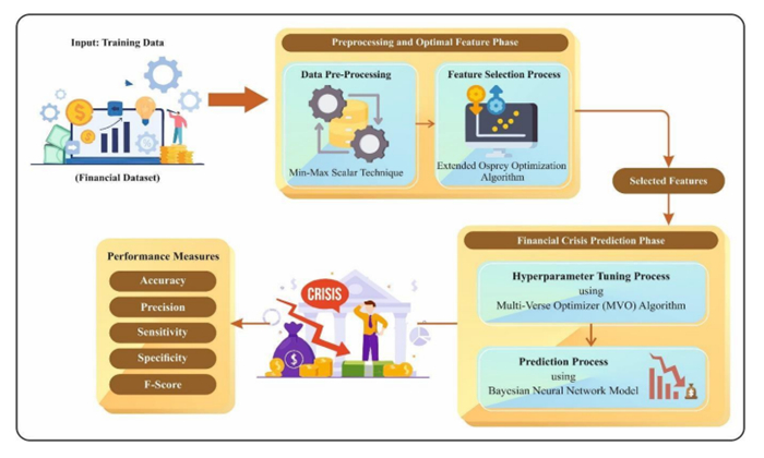
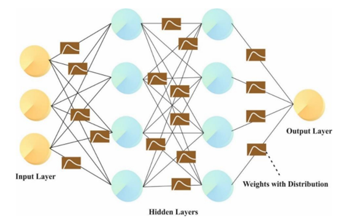
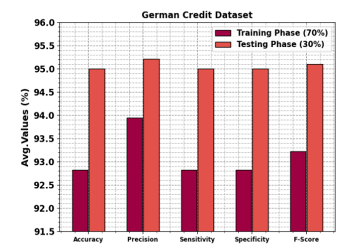
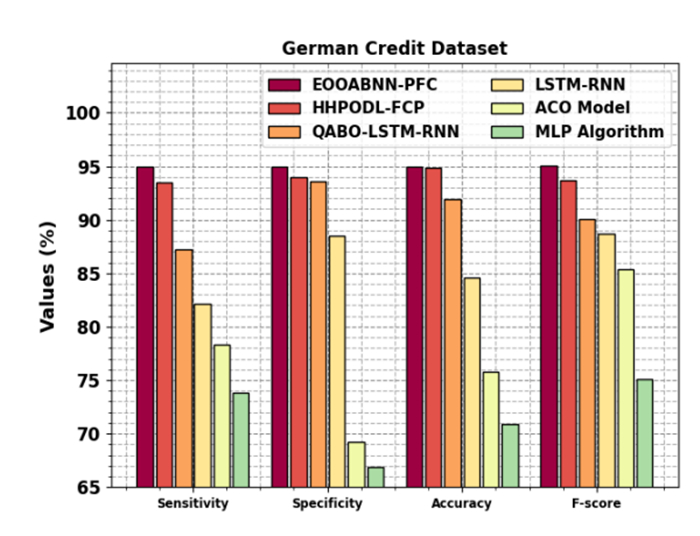
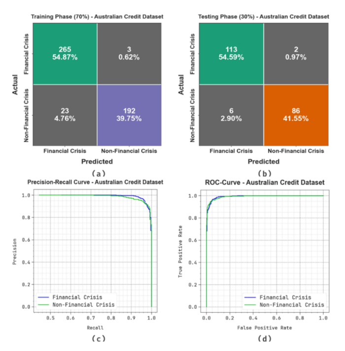
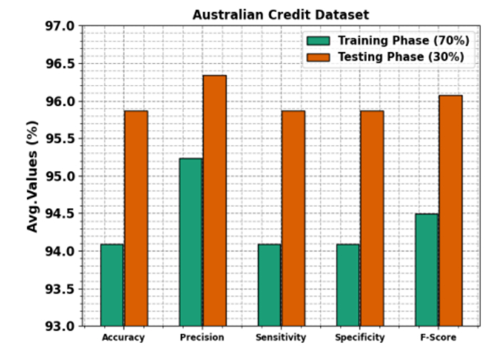
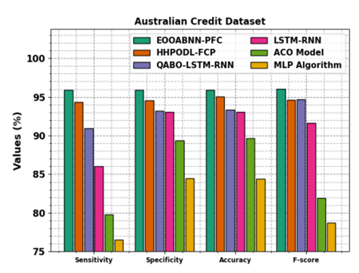
Accurately predicting and anticipating financial crises becomes of paramount importance in the rapidly evolving landscape of financial technology (Fintech). There is an increasing reliance on predictive modeling and advanced analytics techniques to predict possible crises and alleviate the effects of Fintech innovations reshaping traditional financial paradigms. Financial experts and academics are focusing more on financial risk prevention and control tools based on state-of-the-art technology such as machine learning (ML), big data, and neural networks (NN). Researchers aim to prioritize and identify the most informative variables for accurate prediction models by leveraging the abilities of deep learning and feature selection (FS) techniques. This combination of techniques allows the extraction of relationships and nuanced patterns from complex financial datasets, empowering predictive models to discern subtle signals indicative of potential crises. This study developed an extended osprey optimization algorithm with a Bayesian NN to predict financial crisis (EOOABNN-PFC) technique. The EOOABNN-PFC technique uses metaheuristics and the Bayesian model to predict the presence of a financial crisis. In preprocessing, the EOOABNN-PFC technique uses a min-max scalar to scale the input data into a valid format. Besides, the EOOABNN-PFC technique applies the EOOA-based feature subset selection approach to elect the optimal feature subset, and the prediction of the financial crisis is performed using the BNN classifier. Lastly, the optimal parameter selection of the BNN model is carried out using a multi-verse optimizer (MVO). The simulation process identified that the EOOABNN-PFC technique reaches superior accuracy outcomes of 95.00% and 95.87% compared with other existing approaches under the German Credit and Australian Credit datasets.
Citation: Ilyos Abdullayev, Elvir Akhmetshin, Irina Kosorukova, Elena Klochko, Woong Cho, Gyanendra Prasad Joshi. Modeling of extended osprey optimization algorithm with Bayesian neural network: An application on Fintech to predict financial crisis[J]. AIMS Mathematics, 2024, 9(7): 17555-17577. doi: 10.3934/math.2024853
Accurately predicting and anticipating financial crises becomes of paramount importance in the rapidly evolving landscape of financial technology (Fintech). There is an increasing reliance on predictive modeling and advanced analytics techniques to predict possible crises and alleviate the effects of Fintech innovations reshaping traditional financial paradigms. Financial experts and academics are focusing more on financial risk prevention and control tools based on state-of-the-art technology such as machine learning (ML), big data, and neural networks (NN). Researchers aim to prioritize and identify the most informative variables for accurate prediction models by leveraging the abilities of deep learning and feature selection (FS) techniques. This combination of techniques allows the extraction of relationships and nuanced patterns from complex financial datasets, empowering predictive models to discern subtle signals indicative of potential crises. This study developed an extended osprey optimization algorithm with a Bayesian NN to predict financial crisis (EOOABNN-PFC) technique. The EOOABNN-PFC technique uses metaheuristics and the Bayesian model to predict the presence of a financial crisis. In preprocessing, the EOOABNN-PFC technique uses a min-max scalar to scale the input data into a valid format. Besides, the EOOABNN-PFC technique applies the EOOA-based feature subset selection approach to elect the optimal feature subset, and the prediction of the financial crisis is performed using the BNN classifier. Lastly, the optimal parameter selection of the BNN model is carried out using a multi-verse optimizer (MVO). The simulation process identified that the EOOABNN-PFC technique reaches superior accuracy outcomes of 95.00% and 95.87% compared with other existing approaches under the German Credit and Australian Credit datasets.

| [1] |
P. Mohan, S. Neelakandan, A. Mardani, S. Maurya, N. Arulkumar, K. Thangaraj, Eagle strategy arithmetic optimisation algorithm with optimal deep convolutional forest based FinTech application for hyper-automation, Enterp. Inf. Syst., 2023, 2188123. https://doi.org/10.1080/17517575.2023.2188123 doi: 10.1080/17517575.2023.2188123

|
| [2] |
V. Balmaseda, M. Coronado, G. C. Santiagoc, Predicting systemic risk in financial systems using deep graph learning, Intell. Syst. Appl., 19 (2023), 200240. https://doi.org/10.1016/j.iswa.2023.200240 doi: 10.1016/j.iswa.2023.200240
|
| [3] |
J. Uthayakumar, N. Metawa, K. Shankar, S. K. Lakshmanaprabu, An intelligent hybrid model for financial crisis prediction using machine learning techniques, Inf. Syst. E-Bus. Manag., 18 (2020), 617–645. https://doi.org/10.1007/s10257-018-0388-9 doi: 10.1007/s10257-018-0388-9
|
| [4] |
L. Liu, C. Chen, B. Wang, Predicting financial crises with machine learning methods, J. Forecasting, 41 (2022), 871–910. https://doi.org/10.1002/for.2840 doi: 10.1002/for.2840
|
| [5] |
P. Khuwaja, S. A. Khowaja, K. Dev, Adversarial learning networks for Fintech applications using heterogeneous data sources, IEEE Internet Things, 10 (2021), 2194–2201. https://doi.org/10.1109/JIOT.2021.3100742 doi: 10.1109/JIOT.2021.3100742
|
| [6] | M. Bazarbash, Fintech in financial inclusion: Machine learning applications in assessing credit risk, International Monetary Fund, Working Paper, 2019, 1–34. |
| [7] |
B. M. Ceron, M. Monge, Financial technologies (FINTECH) revolution and COVID-19: Time trends and persistence, Rev. Econ. Financ., 13 (2023), 58–64. https://doi.org/10.55365/1923.x2023.21.93 doi: 10.55365/1923.x2023.21.93
|
| [8] |
K. Bluwstein, M. Buckmann, A. Joseph, S. Kapadia, Ö. Şimşek, Credit growth, the yield curve, and financial crisis prediction: Evidence from a machine learning approach, J. Int. Econ., 145 (2023), 103773. https://doi.org/10.1016/j.jinteco.2023.103773 doi: 10.1016/j.jinteco.2023.103773
|
| [9] |
D. Ahelegbey, P. Giudici, V. Pediroda, A network-based fintech inclusion platform, Socio-Econ. Plan. Sci., 87 (2023), 101555. https://doi.org/10.1016/j.seps.2023.101555 doi: 10.1016/j.seps.2023.101555
|
| [10] |
S. K. S. Tyagi, Q. Boyang, An intelligent Internet of things aided financial crisis prediction model in fintech, IEEE Internet Things, 10 (2021), 2183–2193. https://doi.org/10.1109/JIOT.2021.3088753 doi: 10.1109/JIOT.2021.3088753
|
| [11] |
K. Muthukumaran, K. Hariharanath, Deep learning enabled financial crisis prediction models for small-medium sized industries, Intell. Autom. Soft Co., 35 (2023), 101–103. https://doi.org/10.32604/iasc.2023.025968 doi: 10.32604/iasc.2023.025968
|
| [12] |
K. Muthukumaran, K. Hariharanath, V. Haridasan, Feature selection with optimal variational auto encoder for financial crisis prediction, Comput. Syst. Sci. Eng., 45 (2023). https://doi.org/10.32604/csse.2023.030627 doi: 10.32604/csse.2023.030627
|
| [13] | R. Kalaivani, A. Saravanan, Exploiting pattern recognition using chimp optimization algorithm with machine learning for financial crisis prediction, In: 2023 IEEE International Conference on Sustainable Communication Networks and Application (ICSCNA), IEEE, 2023,944–950. https://doi.org/10.1109/ICSCNA58489.2023.10370184 |
| [14] |
A. L. Karn, V. Sachin, S. Sengan, I. Gandhi, L. Ravi, D. K. Sharma, et al., Designing a deep learning-based financial decision support system for Fintech to support corporate customer's credit extension, Malays. J. Comput. Sci., 2022,116–131. https://doi.org/10.22452/mjcs.sp2022no1.9 doi: 10.22452/mjcs.sp2022no1.9
|
| [15] | N. Metawa, M. Elhoseny, A deep learning hybrid optimization model for financial crisis prediction, SSRN Electr. J., 2022, 1–25. http://dx.doi.org/10.2139/ssrn.4167822 |
| [16] |
T. Vaiyapuri, K. Priyadarshini, A. Hemlathadhevi, M. Dhamodaran, A. K. Dutta, I. V. Pustokhina, et al., Intelligent feature selection with deep learning based financial risk assessment model, Comput. Mater. Con., 72 (2022). https://doi.org/10.32604/cmc.2022.026204 doi: 10.32604/cmc.2022.026204
|
| [17] | M. Park, S. Chai, A machine learning-based model for the asymmetric prediction of accounting and financial information, In: Fintech with Artificial Intelligence, Big Data, and Blockchain, Singapore: Springer, 2021,181–190. https://doi.org/10.1007/978-981-33-6137-9-7 |
| [18] |
I. Katib, F. Y. Assiri, T. Althaqafi, Z. M. A. Kubaisy, D. Hamed, M. Ragab, Hybrid hunter-prey optimization with deep learning-based Fintech for predicting financial crises in the economy and society, Electronics, 12 (2023), 3429. https://doi.org/10.3390/electronics12163429 doi: 10.3390/electronics12163429
|
| [19] |
S. Liu, N. Lu, W. Hong, C. Qian, K. Tang, Effective and imperceptible adversarial textual attack via multi-objectivization, ACM T. Evolut. Learn., 2021. https://doi.org/10.1145/3651166 doi: 10.1145/3651166
|
| [20] |
S. Liu, N. Lu, C. Chen, K. Tang, Efficient combinatorial optimization for word-level adversarial textual attack. IEEE-ACM T. Audio Spe., 30 (2021), 98–111. https://doi.org/10.1109/TASLP.2021.3130970 doi: 10.1109/TASLP.2021.3130970
|
| [21] |
C. Huang, Y. Liand, X. Yao, A survey of automatic parameter tuning methods for metaheuristics, IEEE T. Evolut. Comput., 24 (2019), 201–216. https://doi.org/10.1109/TEVC.2019.2921598 doi: 10.1109/TEVC.2019.2921598
|
| [22] | S. Liu, K. Tang, Y. Lei, X. Yao, On performance estimation in automatic algorithm configuration, In: Proceedings of the AAAI Conference on Artificial Intelligence, 34 (2020), https://doi.org/10.1609/aaai.v34i03.5618 |
| [23] |
S. Liu, K. Tang, X. Yao, Generative adversarial construction of parallel portfolios, IEEE T. Cybernetics, 52 (2020), 784–795. https://doi.org/10.1109/TCYB.2020.2984546 doi: 10.1109/TCYB.2020.2984546
|
| [24] |
Z. Guo, Z. Yin, Y. Lyu, Y. Wang, S. Chen, Y. Li, et al., Research on indoor environment prediction of pig house based on OTDBO-TCN-GRU algorithm, Animals, 14 (2024), 863. https://doi.org/10.3390/ani14060863 doi: 10.3390/ani14060863
|
| [25] |
H. A. Ahmed, H. A. A. AL-Asadi, An optimized link state routing protocol with a blockchain framework for efficient video-packet transmission and security over mobile ad-hoc networks, J. Sens. Actuar. Netw., 13 (2024), 22. https://doi.org/10.3390/jsan13020022 doi: 10.3390/jsan13020022
|
| [26] |
H. Yu, A. H. Seno, Z. S. Khodaei, M. F. Aliabadi, Structural health monitoring impact classification method based on Bayesian neural network, Polymers, 14 (2022), 3947. https://doi.org/10.3390/polym14193947 doi: 10.3390/polym14193947
|
| [27] |
H. Gör, Feasibility of six metaheuristic solutions for estimating induction motor reactance, Mathematics, 12 (2024), 483. https://doi.org/10.3390/math12030483 doi: 10.3390/math12030483
|
| [28] | Statlog, German Credit Data, Available from: https://archive.ics.uci.edu/ml/datasets/ statlog+(german+credit+data). https://doi.org/10.24432/C5NC77 |
| [29] | Statlog Australian Credit Approval, Avilable from: http://archive.ics.uci.edu/ml/datasets/ statlog+(australian+credit+approval). https://doi.org/10.24432/C59012 |
Figures(14) / Tables(7)

Ilyos Abdullayev, Elvir Akhmetshin, Irina Kosorukova, Elena Klochko, Woong Cho, Gyanendra Prasad Joshi. Modeling of extended osprey optimization algorithm with Bayesian neural network: An application on Fintech to predict financial crisis[J]. AIMS Mathematics, 2024, 9(7): 17555-17577. doi: 10.3934/math.2024853


 DownLoad: