Reliability analysis at usual operating settings for Weibull Constant-stress model with improved adaptive Type-Ⅱ progressively censored samples

Mazen Nassar; Refah Alotaibi; Ahmed Elshahhat; Mazen Nassar; Refah Alotaibi; Ahmed Elshahhat

doi:10.3934/math.2024823

AIMS Mathematics

2024, Volume 9, Issue 7: 16931-16965. doi: 10.3934/math.2024823

Previous Article Next Article

Research article Special Issues

Reliability analysis at usual operating settings for Weibull Constant-stress model with improved adaptive Type-Ⅱ progressively censored samples

1.
Department of Statistics, Faculty of Science, King Abdulaziz University, Jeddah 21589, Saudi Arabia
2.
Department of Statistics, Faculty of Commerce, Zagazig University, Zagazig 44519, Egypt
3.
Department of Mathematical Sciences, College of Science, Princess Nourah bint Abdulrahman University, P.O. Box 84428, Riyadh 11671, Saudi Arabia
4.
Faculty of Technology and Development, Zagazig University, Zagazig 44519, Egypt

Received: 27 February 2024 Revised: 09 April 2024 Accepted: 06 May 2024 Published: 15 May 2024
MSC : 62F10, 62F15, 62N01, 62N02, 62N05

An improved adaptive Type-Ⅱ progressive censoring scheme was recently introduced to ensure that the examination duration will not surpass a specified threshold span. Employing this plan, this paper aimed to investigate statistical inference using Weibull constant-stress accelerated life tests. Two classical setups, namely maximum likelihood and maximum product of spacings, were explored to estimate the scale, shape, and reliability index under normal use conditions as well as their asymptotic confidence intervals. Through the same suggested classical setups, the Bayesian estimation methodology via the Markov chain Monte Carlo technique based on the squared error loss was considered to acquire the point and credible estimates. To compare the efficiency of the various offered approaches, a simulation study was carried out with varied sample sizes and censoring designs. The simulation findings show that the Bayesian approach via the likelihood function provides better estimates when compared with other methods. Finally, the utility of the proposed techniques was illustrated by analyzing two real data sets indicating the failure times of a white organic light-emitting diode and a pump motor.
Citation: Mazen Nassar, Refah Alotaibi, Ahmed Elshahhat. Reliability analysis at usual operating settings for Weibull Constant-stress model with improved adaptive Type-Ⅱ progressively censored samples[J]. AIMS Mathematics, 2024, 9(7): 16931-16965. doi: 10.3934/math.2024823

Related Papers:

Abstract

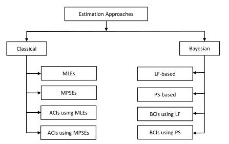
An improved adaptive Type-Ⅱ progressive censoring scheme was recently introduced to ensure that the examination duration will not surpass a specified threshold span. Employing this plan, this paper aimed to investigate statistical inference using Weibull constant-stress accelerated life tests. Two classical setups, namely maximum likelihood and maximum product of spacings, were explored to estimate the scale, shape, and reliability index under normal use conditions as well as their asymptotic confidence intervals. Through the same suggested classical setups, the Bayesian estimation methodology via the Markov chain Monte Carlo technique based on the squared error loss was considered to acquire the point and credible estimates. To compare the efficiency of the various offered approaches, a simulation study was carried out with varied sample sizes and censoring designs. The simulation findings show that the Bayesian approach via the likelihood function provides better estimates when compared with other methods. Finally, the utility of the proposed techniques was illustrated by analyzing two real data sets indicating the failure times of a white organic light-emitting diode and a pump motor.

References

[1]	N. Balakrishnan, D. Han, Exact inference for a simple step-stress model with competing risks for failure from exponential distribution under Type-Ⅱ censoring, J. Stat. Plan. Infer., 138 (2008), 4172–4186. https://doi.org/10.1016/j.jspi.2008.03.036 doi: 10.1016/j.jspi.2008.03.036
[2]	W. B. Nelson, Accelerated Testing: Statistical Models, Test Plans, and Data Analysis, Amsterdam: John Wiley & Sons, 2009.
[3]	M. Kateri, U. Kamps, Inference in step-stress models based on failure rates, Stat. Papers, 56 (2015), 639–660. https://doi.org/10.1007/s00362-014-0601-y doi: 10.1007/s00362-014-0601-y
[4]	M. M. El-Din, S. E. Abu-Youssef, N. S. Ali, A. M. Abd El-Raheem, Estimation in constant-stress accelerated life tests for extension of the exponential distribution under progressive censoring, Metron, 74 (2016), 253–273. https://doi.org/10.1007/s40300-016-0089-4 doi: 10.1007/s40300-016-0089-4
[5]	L. Wang, Estimation of constant-stress accelerated life test for Weibull distribution with nonconstant shape parameter, J. Comput. Appl. Math., 343 (2018), 539–555. https://doi.org/10.1016/j.cam.2018.05.012 doi: 10.1016/j.cam.2018.05.012
[6]	S. G. Nassr, N. M. Elharoun, Inference for exponentiated Weibull distribution under constant stress partially accelerated life tests with multiple censored, Commun. Stat. Appl. Meth., 26 (2019), 131–148. https://doi.org/10.29220/CSAM.2019.26.2.131 doi: 10.29220/CSAM.2019.26.2.131
[7]	M. Nassar, H. Okasha, M. Albassam, E-Bayesian estimation and associated properties of simple step–stress model for exponential distribution based on Type-Ⅱ censoring, Qual. Reliab. Eng. Int., 37 (2021), 997–1016. https://doi.org/10.1002/qre.2778 doi: 10.1002/qre.2778
[8]	M. Nassar, S. Dey, L. Wang, A. Elshahhat, Estimation of Lindley constant-stress model via product of spacing with Type-Ⅱ censored accelerated life data, Commun. Stat. Simul. Comput., 53 (2024), 288–314. https://doi.org/10.1080/03610918.2021.2018460 doi: 10.1080/03610918.2021.2018460
[9]	S. Dey, M. Nassar, Classical methods of estimation on constant stress accelerated life tests under exponentiated Lindley distribution, J. Appl. Stat., 47 (2020), 975–996. https://doi.org/10.1080/02664763.2019.1661361 doi: 10.1080/02664763.2019.1661361
[10]	X. Feng, J. Tang, Q. Tan, Z. Yin, Reliability model for dual constant-stress accelerated life test with Weibull distribution under Type-Ⅰ censoring scheme, Commun. Stat. Theory Meth., 51 (2022), 8579–8597. https://doi.org/10.1080/03610926.2021.1900868 doi: 10.1080/03610926.2021.1900868
[11]	N. Balakrishnan, E. Castilla, M. H. Ling, Optimal designs of constant-stress accelerated life-tests for one-shot devices with model misspecification analysis, Qual. Reliab. Eng. Int., 38 (2022), 989–1012. https://doi.org/10.1002/qre.3031 doi: 10.1002/qre.3031
[12]	R. Alotaibi, M. Nassar, A. Elshahhat, Reliability estimation under normal operating conditions for progressively Type-Ⅱ XLindley censored data, Axioms, 12 (2023), 352. https://doi.org/10.3390/axioms12040352 doi: 10.3390/axioms12040352
[13]	D. Kumar, M. Nassar, S. Dey, F. M. A. Alam, On estimation procedures of constant stress accelerated life test for generalized inverse Lindley distribution, Qual. Reliab. Eng. Int., 38 (2022), 211–228. https://doi.org/10.1002/qre.2971 doi: 10.1002/qre.2971
[14]	M. Y. Manal, R. Alsultan, S. G. Nassr, Parametric inference on partially accelerated life testing for the inverted Kumaraswamy distribution based on Type-Ⅱ progressive censoring data, Math. Biosci. Eng., 20 (2023), 1674–1694. https://doi.org/10.3934/mbe.2023076 doi: 10.3934/mbe.2023076
[15]	W. Wu, B. X. Wang, J. Chen, J. Miao, Q. Gun, Interval estimation of the two-parameter exponential constant stress accelerated life test model under Type-Ⅱ censoring, Qual. Technol. Quant. Manag., 20 (2023), 751–762. https://doi.org/10.1080/16843703.2022.2147688 doi: 10.1080/16843703.2022.2147688
[16]	D. Kundu, A. Joarder, Analysis of Type-Ⅱ progressively hybrid censored data, Comput. Stat. Data Anal., 50 (2006), 2509–2528. https://doi.org/10.1016/j.csda.2005.05.002 doi: 10.1016/j.csda.2005.05.002
[17]	H. K. T. Ng, D. Kundu, P. S. Chan, Statistical analysis of exponential lifetimes under an adaptive Type-Ⅱ progressive censoring scheme, Naval Res. Logist., 56 (2009), 687–698. https://doi.org/10.1002/nav.20371 doi: 10.1002/nav.20371
[18]	A. A. Ismail, Inference for a step-stress partially accelerated life test model with an adaptive Type-Ⅱ progressively hybrid censored data from Weibull distribution, J. Comput. Appl. Math., 260 (2014), 533–542. https://doi.org/10.1016/j.cam.2013.10.014 doi: 10.1016/j.cam.2013.10.014
[19]	M. M. A. Sobhi, A. A. Soliman, Estimation for the exponentiated Weibull model with adaptive Type-Ⅱ progressive censored schemes, Appl. Mathe. Model., 40 (2016), 1180–1192. https://doi.org/10.1016/j.apm.2015.06.022 doi: 10.1016/j.apm.2015.06.022
[20]	M. Nassar, O. E. Abo-Kasem, Estimation of the inverse Weibull parameters under adaptive type-Ⅱ progressive hybrid censoring scheme, J. Comput. Appl. Math., 315 (2017), 228–239. https://doi.org/10.1016/j.cam.2016.11.012 doi: 10.1016/j.cam.2016.11.012
[21]	M. Nassar, O. Abo-Kasem, C. Zhang, S. Dey, Analysis of Weibull distribution under adaptive type-Ⅱ progressive hybrid censoring scheme, J. Indian Soc. Probab. Stat., 19 (2018), 25–65. https://doi.org/10.1007/s41096-018-0032-5 doi: 10.1007/s41096-018-0032-5
[22]	A. Elshahhat, M. Nassar, Bayesian survival analysis for adaptive Type-Ⅱ progressive hybrid censored Hjorth data, Comput. Stat., 36 (2021), 1965–1990. https://doi.org/10.1007/s00180-021-01065-8 doi: 10.1007/s00180-021-01065-8
[23]	W. S. Abu El Azm, R. Aldallal, H. M. Aljohani, S. G. Nassr, Estimations of Competing Lifetime data from Inverse Weibull Distribution Under Adaptive progressively hybrid censored, Math. Biosci. Eng., 19 (2022), 6252–6276. https://doi.org/10.3934/mbe.2022292 doi: 10.3934/mbe.2022292
[24]	S. G. Nassr, W. S. Abu El Azm, E. M. Almetwally, Statistical inference for the extended weibull distribution based on adaptive type-Ⅱ progressive hybrid censored competing risks data, Thailand Stat., 19 (2021), 547–564.
[25]	W. Yan, P. Li, Y. Yu, Statistical inference for the reliability of Burr-XⅡ distribution under improved adaptive Type-Ⅱ progressive censoring, Appl. Math. Model., 95 (2021), 38–52. https://doi.org/10.1016/j.apm.2021.01.050 doi: 10.1016/j.apm.2021.01.050
[26]	I. Elbatal, M. Nassar, A. Ben Ghorbal, L. S. G. Diad, A. Elshahhat, Reliability analysis and its applications for a newly improved Type-Ⅱ adaptive progressive Alpha power exponential censored sample, Symmetry, 15 (2023), 2137. https://doi.org/10.3390/sym15122137 doi: 10.3390/sym15122137
[27]	S. Dutta, S. Kayal, Inference of a competing risks model with partially observed failure causes under improved adaptive type-Ⅱ progressive censoring, Proc. Instit. Mech. Eng. Part O: J. Risk Reliab., 237 (2023), 765–780. https://doi.org/10.1177/1748006X221104555 doi: 10.1177/1748006X221104555
[28]	A. Xu, B. Wang, D. Zhu, J. Pang, X. Lian, Bayesian reliability assessment of permanent magnet brake under small sample size, IEEE Transact. Reliab., 2024, 1–11. https://doi.org/10.1109/TR.2024.3381072
[29]	W. Wang, Z. Cui, R. Chen, Y. Wang, X. Zhao, Regression analysis of clustered panel count data with additive mean models, Stat. Papers, 2023. https://doi.org/10.1007/s00362-023-01511-3 doi: 10.1007/s00362-023-01511-3
[30]	W. Wang, D. B. Kececioglu, Fitting the Weibull log-linear model to accelerated life-test data, IEEE Transact. Reliab., 49 (2000), 217–223. https://doi.org/10.1109/24.877341 doi: 10.1109/24.877341
[31]	S. Roy, Bayesian accelerated life test plans for series systems with Weibull component lifetimes, Appl. Math. Model., 62 (2018), 383–403. https://doi.org/10.1016/j.apm.2018.06.007 doi: 10.1016/j.apm.2018.06.007
[32]	W. Cui, Z. Yan, X. Peng, Statistical analysis for constant-stress accelerated life test with Weibull distribution under adaptive Type-Ⅱ hybrid censored data, IEEE Access, 7 (2019), 165336–165344. https://doi.org/10.1109/ACCESS.2019.2950699 doi: 10.1109/ACCESS.2019.2950699
[33]	A. A. Ismail, Statistical analysis of Type-Ⅰ progressively hybrid censored data under constant-stress life testing model, Phys. A: Stat. Mech. Appl., 520 (2019), 138–150. https://doi.org/10.1016/j.physa.2019.01.004 doi: 10.1016/j.physa.2019.01.004
[34]	B. X. Wang, K. Yu, Z. Sheng, New inference for constant-stress accelerated life tests with Weibull distribution and progressively type-Ⅱ censoring, IEEE Transact. Reliab., 63 (2014), 807–815. https://doi.org/10.1109/TR.2014.2313804 doi: 10.1109/TR.2014.2313804
[35]	A. J. Watkins, A. M. John, On constant stress accelerated life tests terminated by Type Ⅱ censoring at one of the stress levels, J. Stat. Plann. Infer., 138 (2008), 768–786. https://doi.org/10.1016/j.jspi.2007.02.013 doi: 10.1016/j.jspi.2007.02.013
[36]	W. H. Greene, Econometric Analysis, 4 Eds, New York: Prentice-Hall, 2000.
[37]	R. C. H. Cheng, N. A. K. Amin, Estimating parameters in cont.inuous univariate distributions with a shifted origin, J. Royal Stat. Soc.: Ser. B, 45 (1983), 394–403.
[38]	B. Ranneby, The maximum spacing method. An estimation method related to the maximum likelihood method, Scand. J. Stat., 11 (1984), 93–112
[39]	S. Basu, S. K. Singh, U. Singh, Estimation of inverse Lindley distribution using product of spacings function for hybrid censored data, Methodol. Comput. Appl. Probab., 21 (2019), 1377–1394. https://doi.org/10.1007/s11009-018-9676-6 doi: 10.1007/s11009-018-9676-6
[40]	G. Volovskiy, U. Kamps, Maximum product of spacings prediction of future record values, Metrika (2020), 853–868. https://doi.org/10.1007/s00184-020-00767-1 doi: 10.1007/s00184-020-00767-1
[41]	A. Chaturvedi, S. K. Singh, U. Singh, Maximum product spacings estimator for fuzzy data using inverse Lindley distribution, Austrian J. Stat., 52 (2023), 86–103. https://doi.org/10.17713/ajs.v52i2.1395 doi: 10.17713/ajs.v52i2.1395
[42]	R. C. H. Cheng, L. Traylor, Non-regular maximum likelihood problems, J. Royal Stat. Soc. Ser. B, 57 (1995), 3–24. https://doi.org/10.1111/j.2517-6161.1995.tb02013.x doi: 10.1111/j.2517-6161.1995.tb02013.x
[43]	K. Ghosh, S. R. Jammalamadaka, A general estimation method using spacings, J. Stat. Plann. Infer., 93 (2001), 71–82. https://doi.org/10.1016/S0378-3758(00)00160-9 doi: 10.1016/S0378-3758(00)00160-9
[44]	S. Anatolyev, G. Kosenok, An alternative to maximum likelihood based on spacings, Economet. Theory, 21 (2005), 472–476. https://doi.org/10.1017/S0266466605050255 doi: 10.1017/S0266466605050255
[45]	M. Plummer, N. Best, K. Cowles, K. Vines, COOD: convergence diagnosis and output analysis for MCMC, R News, 6 (2006), 7–11.
[46]	A. Henningsen, O. Toomet, MaxLik: a package for maximum likelihood estimation in R, Comput. Stat., 26 (2011), 443–458. https://doi.org/10.1007/s00180-010-0217-1 doi: 10.1007/s00180-010-0217-1
[47]	J. M. Pavia, Testing goodness-of-fit with the kernel density estimator: GoFKernel, J. Stat. Software Code Snippet, 66 (2015), 1–27. https://doi.org/10.18637/jss.v066.c01 doi: 10.18637/jss.v066.c01
[48]	M. Nassar, A. Elshahhat, Statistical analysis of inverse Weibull constant-stress partially accelerated life tests with adaptive progressively type Ⅰ censored data, Mathematics, 11 (2023), 370. https://doi.org/10.3390/math11020370 doi: 10.3390/math11020370
[49]	J. Zhang, G. Cheng, X. Chen, Y. Han, T. Zhou, Y. Qiu, Accelerated life test of white OLED based on lognormal distribution, Indian J. Pure Appl. Phys. (IJPAP), 52 (2015), 671–677.
[50]	C. T. Lin, Y. Y. Hsu, S. Y. Lee, N. Balakrishnan, Inference on constant stress accelerated life tests for log-location-scale lifetime distributions with Type-Ⅰ hybrid censoring, J. Stat. Comput. Simul., 89 (2019), 720–749. https://doi.org/10.1080/00949655.2019.1571591 doi: 10.1080/00949655.2019.1571591

Reader Comments

Your name:*

Email:*
© 2024 the Author(s), licensee AIMS Press. This is an open access article distributed under the terms of the Creative Commons Attribution License (http://creativecommons.org/licenses/by/4.0)