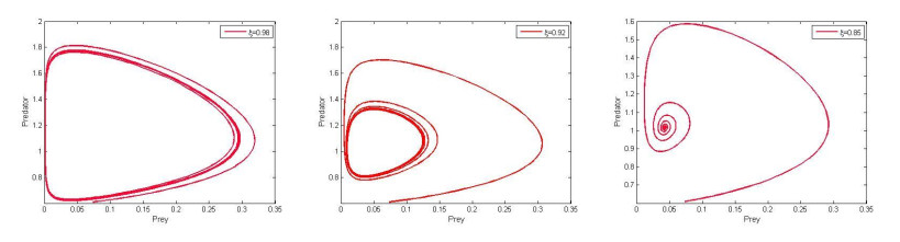
The main objective of our research was to explore and develop a fractional-order derivative within the predator-prey framework. The framework includes prey refuge and selective nonlinear harvesting, where the harvesting progressively approaches a threshold value as the density of the harvested population advances. For memory effect, a non-integer order derivative is better than an integer-order derivative. The solutions to the fractional framework were shown to be existence, uniqueness, non-negativity, and boundedness. Matignon's condition was used for analysing local stability, and a suitable Lyapunov function provided global stability. While discussing the Hopf bifurcation's existence condition, we explored derivative order and refuge as bifurcation parameters. We aimed at redefining the predator-prey framework to incorporate fractional order, refuge, and harvesting. This kind of nonlinear harvesting is more realistic and reasonable than the model with constant yield harvesting and constant effort harvesting. The Adams-Bashforth-Moulton PECE algorithm in MATLAB software was used to simulate the proposed outcomes, investigate the impact on various factors, and analyse harvesting's effect on non-integer order predator-prey interactions.
Citation: Kottakkaran Sooppy Nisar, G Ranjith Kumar, K Ramesh. The study on the complex nature of a predator-prey model with fractional-order derivatives incorporating refuge and nonlinear prey harvesting[J]. AIMS Mathematics, 2024, 9(5): 13492-13507. doi: 10.3934/math.2024657
The main objective of our research was to explore and develop a fractional-order derivative within the predator-prey framework. The framework includes prey refuge and selective nonlinear harvesting, where the harvesting progressively approaches a threshold value as the density of the harvested population advances. For memory effect, a non-integer order derivative is better than an integer-order derivative. The solutions to the fractional framework were shown to be existence, uniqueness, non-negativity, and boundedness. Matignon's condition was used for analysing local stability, and a suitable Lyapunov function provided global stability. While discussing the Hopf bifurcation's existence condition, we explored derivative order and refuge as bifurcation parameters. We aimed at redefining the predator-prey framework to incorporate fractional order, refuge, and harvesting. This kind of nonlinear harvesting is more realistic and reasonable than the model with constant yield harvesting and constant effort harvesting. The Adams-Bashforth-Moulton PECE algorithm in MATLAB software was used to simulate the proposed outcomes, investigate the impact on various factors, and analyse harvesting's effect on non-integer order predator-prey interactions.

| [1] |
P. A. Abrams, Implications of dynamically variable traits for identifying, classifying, and measuring direct and indirect effects in ecological communities, Am. Nat., 146 (1995), 112–134. https://doi.org/10.1086/285789 doi: 10.1086/285789

|
| [2] | E. L. Preisser, D. I. Bolnick, M. F. Benard, Scared to death? The effects of intimidation and consumption in predator-prey interactions, Ecology, 86 (2005), 501–509. |
| [3] |
S. L. Lima, Nonlethal effects in the ecology of predator-prey interactions, Bioscience, 48 (1998), 25–34. https://doi.org/10.2307/1313225 doi: 10.2307/1313225
|
| [4] |
X. Wang, L. Zanette, X. Zou, Modelling the fear effect in predator-prey interactions, J. Math. Biol., 73 (2016), 1179–1204. https://doi.org/10.1007/s00285-016-0989-1 doi: 10.1007/s00285-016-0989-1
|
| [5] |
H. Zhang, Y. Cai, S. Fu, W. Wang, Impact of the fear effect in a prey-predator model incorporating a prey refuge, Appl. Math. Comput., 356 (2019), 328–337. https://doi.org/10.1016/j.amc.2019.03.034 doi: 10.1016/j.amc.2019.03.034
|
| [6] |
S. Chakraborty, S. Pal, N. Bairagi, Predator-prey interaction with harvesting: Mathematical study with biological ramifications, Appl. Math. Model., 36 (2012), 4044–4059. https://doi.org/10.1016/j.apm.2011.11.029 doi: 10.1016/j.apm.2011.11.029
|
| [7] |
K. S. Chaudhuri, S. S. Ray, On the combined harvesting of a prey-predator system, J. Biol. Syst., 4 (1996), 373–389. https://doi.org/10.1142/S0218339096000 doi: 10.1142/S0218339096000
|
| [8] |
D. Xiao, W. Li, M. Han, Dynamics in a ratio-dependent predator-prey model with predator harvesting, J. Math. Anal. Appl., 324 (2006), 14–29. https://doi.org/10.1016/j.jmaa.2005.11.048 doi: 10.1016/j.jmaa.2005.11.048
|
| [9] |
Z. Bi, S. Liu, M. Ouyang, X. Wu, Pattern dynamics analysis of spatial fractional predator-prey system with fear factor and refuge, Nonlinear Dynam., 111 (2023), 10653–10676. https://doi.org/10.1007/s11071-023-08353-6 doi: 10.1007/s11071-023-08353-6
|
| [10] |
B. Mondal, S. Roy, U. Ghosh, P. K. Tiwari, A systematic study of autonomous and non autonomous predator-prey models for the combined effects of fear, refuge, cooperation and harvesting, Eur. Phys. J. Plus, 137 (2022), 724. https://doi.org/10.1140/epjp/s13360-022-02915-0 doi: 10.1140/epjp/s13360-022-02915-0
|
| [11] |
Z. Wei, F. Chen, Dynamics of a delayed predator-prey model with prey refuge, Allee effect and fear effect, Int. J. Bifurc. Chaos, 33 (2023), 2350036. https://doi.org/10.1142/S0218127423500360 doi: 10.1142/S0218127423500360
|
| [12] |
S. Khajanchi, S. Banerjee, Role of constant prey refuge on stage structure predator-prey model withratio dependent functional response, Appl. Math. Comput., 314 (2017), 193–198. https://doi.org/10.1016/j.amc.2017.07.017 doi: 10.1016/j.amc.2017.07.017
|
| [13] |
J. Wang, Y. Cai, S. Fu, W. Wang, The effect of the fear factor on the dynamics of a predator-prey model incorporating the prey refuge, Chaos Int. J. Nonlinear Sci., 29 (2019), 083109. https://doi.org/10.1063/1.5111121 doi: 10.1063/1.5111121
|
| [14] |
K. Sarkar, S. Khajanchi, An eco-epidemiological model with the impact of fear, Chaos Int. J. Nonlinear Sci., 32 (2022), 083126. https://doi.org/10.1063/5.0099584 doi: 10.1063/5.0099584
|
| [15] |
S. Biswas, B. Ahmad, S. Khajanchi, Exploring dynamical complexity of a cannibalistic eco-epidemiological model with multiple time delay, Math. Method. Appl. Sci., 46 (2023), 4184–4211. https://doi.org/10.1002/mma.8749 doi: 10.1002/mma.8749
|
| [16] |
K. Sarkar, S. Khajanchi, Spatiotemporal dynamics of a predator-prey system with fear effect, J. Frankl. I., 360 (2023), 7380–7414. https://doi.org/10.1016/j.jfranklin.2023.05.034 doi: 10.1016/j.jfranklin.2023.05.034
|
| [17] |
C. C. García, Bifurcations in a Leslie-Gower model with constant and proportional prey refuge at high and low density, Nonlinear Anal.-Real, 72 (2023), 103861. https://doi.org/10.1016/j.nonrwa.2023.103861 doi: 10.1016/j.nonrwa.2023.103861
|
| [18] |
C. C. García, Impact of prey refuge in a discontinuous Leslie-Gower model with harvesting and alternative food for predators and linear functional response, Math. Comput. Simulat., 206 (2023), 147–165. https://doi.org/10.1016/j.matcom.2022.11.013 doi: 10.1016/j.matcom.2022.11.013
|
| [19] |
C. Maji, Impact of fear effect in a fractional-order predator-prey system incorporating constant prey refuge, Nonlinear Dynam., 107 (2022), 1329–1342. https://doi.org/10.1007/s11071-021-07031-9 doi: 10.1007/s11071-021-07031-9
|
| [20] |
T. K. Kar, Modelling and analysis of a harvested prey-predator system incorporating a prey refuge, J. Comput. Appl. Math., 185 (2006), 19–33. https://doi.org/10.1016/j.cam.2005.01.035 doi: 10.1016/j.cam.2005.01.035
|
| [21] |
B. Mukhopadhyay, R. Bhattacharyya, Effects of harvesting and predator interference in a model of two-predators competing for a single prey, Appl. Math. Model., 40 (2016), 3264–3274. https://doi.org/10.1016/j.apm.2015.10.018 doi: 10.1016/j.apm.2015.10.018
|
| [22] |
J. Hoekstra, J. C. J. M. van den Bergh, Harvesting and conservation in a predator-prey system, J. Econ. Dyn. Control, 29 (2005), 1097–1120. https://doi.org/10.1016/j.jedc.2004.03.006 doi: 10.1016/j.jedc.2004.03.006
|
| [23] |
A. Suryanto, I. Darti, S. Anam, Stability analysis of a fractional order modified Leslie-Gower model with additive Allee effect, Int. J. Math. Math. Sci., 2017 (2017), 1–9. https://doi.org/10.1155/2017/8273430 doi: 10.1155/2017/8273430
|
| [24] |
Z. Li, L. Liu, S. Dehghan, Y. Chen, D. Xue, A review and evaluation of numerical tools for fractional calculus and fractional order controls, Int. J. Control, 90 (2017), 1165–1181. https://doi.org/10.1080/00207179.2015.1124290 doi: 10.1080/00207179.2015.1124290
|
| [25] | J. Liouville, Sur le calcul des differentielles a indices quelconques, 1832. Available from: https://books.google.com/books?id = 6jfBtwAACAAJ. |
| [26] | S. G. Samko, A. A. Kilbas, O. I. Marichev, Fractional integrals and derivatives: Theory and applications, Switzerland/Philadelphia: Gordon and Breach Science Publishers, 1993. |
| [27] |
G. A. Farid, Unified integral operator and further its consequences, Open. J. Math. Anal., 4 (2020), 1–7. https://doi:10.30538/psrp-oma2020.0047 doi: 10.30538/psrp-oma2020.0047
|
| [28] |
H. S. Panigoro, E. Rahmi, N. Achmad, S. L. Mahmud, The influence of additive Allee effect and periodic harvesting to the dynamics of Leslie-Gower predator-prey model, Jambura J. Math., 2 (2020), 87–96. https://doi.org/10.34312/jjom.v2i2.4566 doi: 10.34312/jjom.v2i2.4566
|
| [29] |
H. S. Panigoro, A. Suryanto, W. M. Kusumawinahyu, I. Darti, Dynamics of an eco-epidemic predator-prey model involving fractional derivatives with power-law and Mittag-Leffler kernel, Symmetry., 13 (2021), 785. https://doi.org/10.3390/sym13050785 doi: 10.3390/sym13050785
|
| [30] |
E. Rahmi, I. Darti, A. Suryanto, Trisilowati, A modified Leslie-Gower model incorporating Beddington-Deangelis functional response, double Allee effect and memory effect, Fractal Fract., 5 (2021), 84. https://doi.org/10.3390/fractalfract5030084 doi: 10.3390/fractalfract5030084
|
| [31] |
M. Alqhtani, K. M. Owolabi, K. M. Saad, Spatiotemporal (target) patterns in sub-diffusive predator-prey system with the Caputo operator, Chaos Soliton. Fract., 160 (2022), 112267. https://doi.org/10.1016/j.chaos.2022.112267 doi: 10.1016/j.chaos.2022.112267
|
| [32] |
A. Waleed, Y. A. Amer, E. S. M. Youssef, A. M. S. Mahdy, Mathematical analysis and simulations for a Caputo-Fabrizio fractional COVID-19 model, Partial Differ. Eq. Appl. Math., 8 (2023), 100558. https://doi.org/10.1016/j.padiff.2023.100558 doi: 10.1016/j.padiff.2023.100558
|
| [33] |
S. A. M Abdelmohsen, D. S. Mohamed, H. A. Alyousef, M. R. Gorji, A. M. S. Mahdy, Mathematical modeling for solving fractional model cancer bosom malignant growth, AIMS Biophys., 10 (2023), 263–280. https://doi:10.3934/biophy.2023018 doi: 10.3934/biophy.2023018
|
| [34] |
A. M. S. Mahdy, D. S. Mohamed, Approximate solution of Cauchy integral equations by using Lucas polynomials, Comput. Appl. Math., 41 (2022), 403. https://doi.org/10.1007/s40314-022-02116-6 doi: 10.1007/s40314-022-02116-6
|
| [35] |
A. G. Khaled, S. M. Mohamed, A. Hammad, A. M. S. Mahdy, Dynamical behaviors of nonlinear coronavirus (COVID-19) model with numerical studies, CMC-Comput. Mater. Con., 67 (2021), 675–686. https://doi.org/10.32604/cmc.2021.012200 doi: 10.32604/cmc.2021.012200
|
| [36] | D. Matignon, Stability results for fractional differential equations with applications to control processing, Comput. Eng. Syst. Appl., 2 (1996), 963–968. |
| [37] | I. Petráš, Fractional-order nonlinear systems: Modeling, analysis and simulation, Berlin: Springer, 2011. https://doi.org/10.1007/978-3-642-18101-6 |
| [38] |
Z. M. Odibat, N. T. Shawagfeh, Generalized Taylor's formula, Appl. Math. Comput., 186 (2007), 286–293. https://doi.org/10.1016/j.amc.2006.07.102 doi: 10.1016/j.amc.2006.07.102
|
| [39] |
Y. Li, Y. Chen, I. Podlubny, Stability of fractional-order nonlinear dynamic systems: Lyapunov direct method and generalized Mittag-Leffler stability, Comput. Math. Appl., 59 (2010), 1810–1821. https://doi.org/10.1016/j.camwa.2009.08.019 doi: 10.1016/j.camwa.2009.08.019
|
| [40] |
H. Li, L. Zhang, C. Hu, Y. Jiang, Z. Teng, Dynamical analysis of a fractional-order predator-prey model incorporating a prey refuge, J. Appl. Math. Comput., 54 (2017), 435–449. https://doi.org/10.1007/s12190-016-1017-8 doi: 10.1007/s12190-016-1017-8
|
| [41] |
S. K. Choi, B. Kang, N. Koo, Stability for Caputo fractional differential systems, Abstr. Appl. Anal., 2014 (2014), 1–6. https://doi.org/10.1155/2014/631419 doi: 10.1155/2014/631419
|
| [42] |
C. Vargas-De-Leon, Volterra-type Lyapunov functions for fractional-order epidemic systems, Commun. Nonlinear Sci., 24 (2015), 75–85. https://doi.org/10.1016/j.cnsns.2014.12.013 doi: 10.1016/j.cnsns.2014.12.013
|
| [43] |
J. Huo, H. Zhao, L. Zhu, The effect of vaccines on backward bifurcation in a fractional order HIV model, Nonlinear Anal.-Real, 26 (2015), 289–305. https://doi.org/10.1016/j.nonrwa.2015.05.014 doi: 10.1016/j.nonrwa.2015.05.014
|
| [44] |
M. S. Abdelouahab, N. Hamri, J. Wang, Hopf bifurcation and chaos in fractional-ordermodified hybrid optical system, Nonlinear Dynam., 69 (2012), 275–284. https://doi.org/10.1007/s11071-011-0263-4 doi: 10.1007/s11071-011-0263-4
|
| [45] |
X. Li, R. Wu, Hopf bifurcation analysis of a new commensurate fractional-order hyperchaotic system, Nonlinear Dynam., 78 (2014), 279–288. https://doi.org/10.1007/s11071-014-1439-5 doi: 10.1007/s11071-014-1439-5
|


Figures(6)

Kottakkaran Sooppy Nisar, G Ranjith Kumar, K Ramesh. The study on the complex nature of a predator-prey model with fractional-order derivatives incorporating refuge and nonlinear prey harvesting[J]. AIMS Mathematics, 2024, 9(5): 13492-13507. doi: 10.3934/math.2024657


 DownLoad: