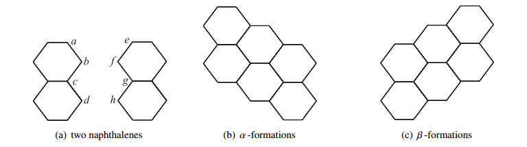
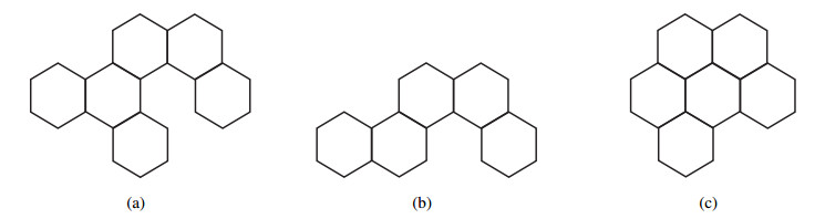
Polycyclic aromatic hydrocarbon (PAH) is a compound composed of carbon and hydrogen atoms. Chemically, large PAHs contain at least two benzene rings and exist in a linear, cluster, or angular arrangement. Hexagonal systems are a typical class of PAHs. The Clar covering polynomial of hexagonal systems contains many important topological properties of condensed aromatic hydrocarbons, such as Kekulé number, Clar number, first Herndon number, which is an important theoretical quantity for predicting the aromatic stability of PAH conjugation systems, and so on. In this paper, we first obtained some recursive formulae for the Clar covering polynomials of double hexagonal chains and proposed a Matlab algorithm to compute the Clar covering polynomial of any double hexagonal chain. Moreover, we presented the characterization of extremal double hexagonal chains with maximum and minimum Clar covering polynomials in all double hexagonal chains with fixed $ s $ naphthalenes.
Citation: Peirong Li, Hong Bian, Haizheng Yu, Yan Dou. Clar covering polynomials of polycyclic aromatic hydrocarbons[J]. AIMS Mathematics, 2024, 9(5): 13385-13409. doi: 10.3934/math.2024653
Polycyclic aromatic hydrocarbon (PAH) is a compound composed of carbon and hydrogen atoms. Chemically, large PAHs contain at least two benzene rings and exist in a linear, cluster, or angular arrangement. Hexagonal systems are a typical class of PAHs. The Clar covering polynomial of hexagonal systems contains many important topological properties of condensed aromatic hydrocarbons, such as Kekulé number, Clar number, first Herndon number, which is an important theoretical quantity for predicting the aromatic stability of PAH conjugation systems, and so on. In this paper, we first obtained some recursive formulae for the Clar covering polynomials of double hexagonal chains and proposed a Matlab algorithm to compute the Clar covering polynomial of any double hexagonal chain. Moreover, we presented the characterization of extremal double hexagonal chains with maximum and minimum Clar covering polynomials in all double hexagonal chains with fixed $ s $ naphthalenes.

| [1] |
H. Zhang, F. Zhang, The Clar covering polynomial of hexagonal systems Ⅰ, Discrete Appl. Math., 69 (1996), 147–167. https://doi.org/10.1016/0166-218X(95)00081-2 doi: 10.1016/0166-218X(95)00081-2

|
| [2] | S. J. Cyvin, I. Gutman, Kekulé structures in benzenoid hydrocarbons, Heidelberg: Springer Berlin, 1988. https://doi.org/10.1007/978-3-662-00892-8 |
| [3] | D. Vukičević, H. W. Kroto, M. Randić, Atlas Kekuléovih valentnih struktura Buckminsterfulerena, Croat. Chem. Acta, 78 (2005), 223–234. |
| [4] |
A. T. Balaban, M. Pompe, M. Randić, $\pi$-Electron partitions, signatures, and Clar structures of selected benzenoid hydrocarbons, J. Phys. Chem., 112 (2008), 4148–4157. https://doi.org/10.1021/jp800246d doi: 10.1021/jp800246d
|
| [5] |
Z. Rashid, J. H, Van Lenthe, R. W. A. Havenith, Resonance and aromaticity: An ab initio valence bond approach, J. Phys. Chem., 116 (2012), 4778–4788. https://doi.org/10.1021/jp211105t doi: 10.1021/jp211105t
|
| [6] | I. Gutman, S. J. Cyvin, Introduction to the theory of benzenoid hydrocarbons, Heidelberg: Springer Berlin, 1989. https://doi.org/10.1007/978-3-642-87143-6 |
| [7] |
F. J. Zhang, H. P. Zhang, Y. T. Liu The Clar covering polynomial of hexagonal systems Ⅱ. An application to resonance energy of condensed aromatic hydrocarbons, Chinese J. Chem., 14 (1996), 321–325. https://doi.org/10.1002/cjoc.19960140407 doi: 10.1002/cjoc.19960140407
|
| [8] |
H. P. Zhang, F. J. Zhang, The Clar covering polynomial of hexagonal systems Ⅲ, Discrete Math., 212 (2000), 261–269. https://doi.org/10.1016/S0012-365X(99)00293-9 doi: 10.1016/S0012-365X(99)00293-9
|
| [9] |
S. Klavžar, P. žigert, I. Gutman, Clar number of catacondensed benzenoid hydrocarbons, J. Mol. Struc. Theochem, 586 (2002), 235–240. https://doi.org/10.1016/S0166-1280(02)00069-6 doi: 10.1016/S0166-1280(02)00069-6
|
| [10] | S. Gojak, S. Stanković, I. Gutman, B. Furtula, Zhang-Zhang polynomial and some of its applications, Math. Method. Chem., 2006,141–158. |
| [11] |
S. Zhou, H. Zhang, I. Gutman, Relations between Clar structures, Clar covers, and the sextet-rotation tree of a hexagonal system, Discrete. Appl. Math., 156 (2008), 1809–1821. https://doi.org/10.1016/j.dam.2007.08.047 doi: 10.1016/j.dam.2007.08.047
|
| [12] |
W. C. Herndon, Resonance energies of aromatic hydrocarbons. Quantitative test of resonance theory, J. Am. Chem. Soc., 95 (1973), 2404–2406. https://doi.org/10.1021/ja00788a073 doi: 10.1021/ja00788a073
|
| [13] |
R. Swinborne-Sheldrake, W. C. Herndon, I. Gutman, Kekulé structures and resonance energies of benzenoid hydrocarbons, Tetrahedron Lett., 16 (1975), 755–758. https://doi.org/10.1016/S0040-4039(00)71975-7 doi: 10.1016/S0040-4039(00)71975-7
|
| [14] |
I. Gutman, S. Gojak, B. Furtula, Clar theory and resonance energy, Chem. Phys. Lett., 413 (2005), 396–399. https://doi.org/10.1016/j.cplett.2005.08.010 doi: 10.1016/j.cplett.2005.08.010
|
| [15] |
I. Gutman, S. Gojak, S. Stanković, B. Furtula, A concealed difference between the structure-dependence of Dewar and topological resonance energy, J. Mol. Struc. Theochem, 757 (2005), 119–123. https://doi.org/10.1016/j.theochem.2005.09.012 doi: 10.1016/j.theochem.2005.09.012
|
| [16] |
I. Gutman, S. Gojak, B. Furtula, S. Radenković, A. Vodopivec, Relating total $\pi$-electron energy and resonance energy of benzenoid molecules with Kekulé-and Clar-structure-based parameters, Monatsh. Chem., 137 (2006), 1127–1138. https://doi.org/10.1007/s00706-006-0522-0 doi: 10.1007/s00706-006-0522-0
|
| [17] |
S. Gojak, S. Radenković, R. Kovačević, S. Stanković, J. Durdević, I. Gutman, A difference between the $\pi$-electron properties of catafusenes and perifusenes, Polycycl Aromat. Comp., 26 (2006), 197–206. https://doi.org/10.1080/10406630600760568 doi: 10.1080/10406630600760568
|
| [18] |
S. Gojak, I. Gutman, S. Radenković, A. Vodopivec, Relating resonance energy with the Zhang-Zhang polynomial, J. Serb. Chem. Soc., 72 (2007), 665–671. https://doi.org/10.2298/JSC0707665G doi: 10.2298/JSC0707665G
|
| [19] |
M. Randić, A. T. Balaban, Partitioning of $\pi$-electrons in rings for Clar structures of benzenoid hydrocarbons, J. Chem. Inf. Model., 46 (2006), 57–64. https://doi.org/10.1021/ci050196s doi: 10.1021/ci050196s
|
| [20] |
I. Gutman, B. Borovićanin, Zhang-Zhang polynomial of multiple linear hexagonal chains, Z. Naturforsch. A, 61 (2006), 73–77. https://doi.org/10.1515/zna-2006-1-211 doi: 10.1515/zna-2006-1-211
|
| [21] |
Q. Guo, H. Deng, D. Chen, Zhang-Zhang polynomials of cyclo-polyphenacenes, J. Math. Chem., 46 (2009), 347–362. https://doi.org/10.1007/s10910-008-9466-4 doi: 10.1007/s10910-008-9466-4
|
| [22] |
A. Misra, D. J. Klein, T. Morikawa, Clar theory for molecular benzenoids, J. Phys. Chem. A, 113 (2009), 1151–1158. https://doi.org/10.1021/jp8038797 doi: 10.1021/jp8038797
|
| [23] | C. P. Chou, H. A. Witek, An algorithm and FORTRAN program for automatic computation of the Zhang-Zhang polynomial of benzenoids, Match-Commun. Math. Co., 68 (2012), 3–30. |
| [24] | C. P. Chou, Y. Li, H. A. Witek, Zhang-Zhang polynomials of various classes of benzenoid systems, Match-Commun. Math. Co., 68 (2012), 31-64. |
| [25] |
C. P. Chou, H. A. Witek, Comment on "Zhang-Zhang polynomials of cyclo-polyphenacenes" by Q. Guo, H. Deng and D. Chen, J. Math. Chem., 50 (2012), 1031–1033. https://doi.org/10.1007/s10910-011-9969-2 doi: 10.1007/s10910-011-9969-2
|
| [26] |
C. P. Chou, J. S. Kang, H. A. Witek, Closed-form formulas for the Zhang-Zhang polynomials of benzenoid structures: Prolate rectangles and their generalizations, Discrete Appl. Math., 198 (2016), 101–108. https://doi.org/10.1016/j.dam.2015.06.020 doi: 10.1016/j.dam.2015.06.020
|
| [27] |
N. Bašić, I. Estélyi, R. škrekovski, N. Tratnik, On the Clar number of benzenoid graphs, Match-Commun. Math. Co., 80 (2018), 173–188. https://doi.org/10.48550/arXiv.1709.04195 doi: 10.48550/arXiv.1709.04195
|
| [28] | A. T. Balaban, M. Randić, Coding canonical Clar structures of polycyclic benzenoid hydrocarbons, Match-Commun. Math. Co., 82 (2019), 139–162. |
| [29] | J. Langner, H. Witek, Interface theory of benzenoids, Match-Commun. Math. Co., 84 (2020), 143–176. |
| [30] | G. Li, Y. Pei, Y. Wang, Clar covering polynomials with only real zeros, Match-Commun. Math. Co., 84 (2020), 217–228. |
| [31] |
D. Plavšić, S. Nikolić, N. Trinajstić, The conjugated-circuit model: Application to nonalternant hydrocarbons and a comparison with some other theoretical models of aromaticity, J. Mol. Struc. Theochem, 277 (1992), 213–237. https://doi.org/10.1016/0166-1280(92)87141-L doi: 10.1016/0166-1280(92)87141-L
|
| [32] | P. ž. Pleteršek, Equivalence of the generalized Zhang-Zhang polynomial and the generalized cube polynomial, 2016. https://doi.org/10.48550/arXiv.1612.02986 |
| [33] |
B. Furtula, S. Radenković, I. Redžepović, N. Tratnik, P. Ž. Pleteršek, The generalized Zhang-Zhang polynomial of benzenoid systems-theory and applications, Appl. Math. Comput., 418 (2022), 126822. https://doi.org/10.1016/j.amc.2021.126822 doi: 10.1016/j.amc.2021.126822
|
| [34] |
S. Radenković, I. Redžepović, S. Dordević, B. Furtula, N. Tratnik, P. Ž. Pleteršek, Relating vibrational energy with Kekulé- and Clar-structure-based parameters, Int. J. Quantum Chem., 122 (2022), e26867. https://doi.org/10.1002/qua.26867 doi: 10.1002/qua.26867
|
| [35] |
H. Zhang, The Clar covering polynomial of hexagonal systems with an application to chromatic polynomials, Discrete. Math., 172 (1997), 163–173. https://doi.org/10.1016/S0012-365X(96)00279-8 doi: 10.1016/S0012-365X(96)00279-8
|
| [36] | H. Zhang, W. C. Shiu, P. K. Sun, A relation between Clar covering polynomial and cube polynomial, 2012. https://doi.org/10.48550/arXiv.1210.5322 |
| [37] |
I. Gutman, M. Randić, A. T. Balaban, B. Furtula, V. Vuĉković, $\pi$-electron contents of rings in the double-hexagonal-chain homologous series (pyrene, anthanthrene and other acenoacenes), Polycycl. Aromat. Comp., 25 (2005), 215–226. https://doi.org/10.1080/10406630591007080 doi: 10.1080/10406630591007080
|
| [38] |
M. Alishahi, S. H. Shalmaee, On the edge eccentric and modified edge eccentric connectivity indices of linear benzenoid chains and double hexagonal chains, J. Mol. Struct., 1204 (2020), 127446. https://doi.org/10.1016/j.molstruc.2019.127446 doi: 10.1016/j.molstruc.2019.127446
|
| [39] |
H. Ren, F. Zhang, Double hexagonal chains with maximal Hosoya index and minimal Merrifield-Simmons index, J. Math. Chem., 42 (2007), 679–690. https://doi.org/10.1007/s10910-005-9024-2 doi: 10.1007/s10910-005-9024-2
|
| [40] |
H. Ren, F. Zhang, Double hexagonal chains with minimal total $\pi$-electron energy, J. Math. Chem., 42 (2007), 1041–1056. https://doi.org/10.1007/s10910-006-9159-9 doi: 10.1007/s10910-006-9159-9
|
| [41] |
H. Ren, F. Zhang, Extremal double hexagonal chains with respect to $k$-matchings and $k$-independent sets, Discrete. Appl. Math., 155 (2007), 2269–2281. https://doi.org/10.1016/j.dam.2007.06.003 doi: 10.1016/j.dam.2007.06.003
|
| [42] |
H. Ren, F. Zhang, Double hexagonal chains with maximal energy, Int. J. Quantum Chem., 107 (2007), 1437–1445. https://doi.org/10.1002/qua.21256 doi: 10.1002/qua.21256
|
| [43] | J. A. Bondy, U. S. R. Murty, Graph theory with applications, London: Macmillan, 1976. |
Figures(21) / Tables(5)

Peirong Li, Hong Bian, Haizheng Yu, Yan Dou. Clar covering polynomials of polycyclic aromatic hydrocarbons[J]. AIMS Mathematics, 2024, 9(5): 13385-13409. doi: 10.3934/math.2024653


 DownLoad: