Cardinality bounds on subsets in the partition resolving set for complex convex polytope-like graph

Ali N. A. Koam; Adnan Khalil; Ali Ahmad; Muhammad Azeem; Ali N. A. Koam; Adnan Khalil; Ali Ahmad; Muhammad Azeem

doi:10.3934/math.2024493

AIMS Mathematics

2024, Volume 9, Issue 4: 10078-10094. doi: 10.3934/math.2024493

Previous Article Next Article

Research article

Cardinality bounds on subsets in the partition resolving set for complex convex polytope-like graph

1.
Department of Mathematics, College of Science, Jazan University, P.O. Box 114, Jazan 45142, Saudi Arabia
2.
Department of Computer Sciences, Al-Razi Institute Saeed Park, Lahore, Pakistan
3.
Department of Information Technology and Security, College of Computer Science and Information Technology, Jazan University, Jazan, Saudi Arabia
4.
Department of Mathematics, Riphah International University, Lahore, Pakistan

Received: 06 November 2023 Accepted: 02 January 2024 Published: 13 March 2024
MSC : 05C09, 05C35, 05C38, 05C72, 05C76

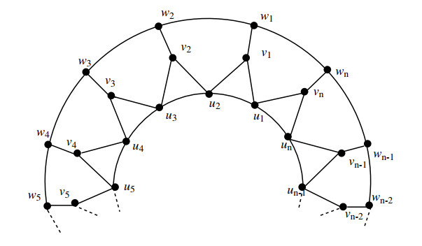
Let $ G = (V, E) $ be a simple, connected graph with vertex set $ V(G) $ and $ E(G) $ edge set of $ G $. For two vertices $ a $ and $ b $ in a graph $ G $, the distance $ d(a, b) $ from $ a $ to $ b $ is the length of shortest path $ a-b $ path in $ G $. A $ k $-ordered partition of vertices of $ G $ is represented as $ {R}{p} = \{{R}{p_1}, {R}{p_2}, \dots, {R}{p_k}\} $ and the representation $ r(a|{R}{p}) $ of a vertex $ a $ with respect to $ {R}{p} $ is the vector $ (d(a|{R}{p_1}), d(a|{R}{p_2}), \dots, d(a|{R}{p_k})) $. The partition is called a resolving partition of $ G $ if $ r(a|{R}{p}) \ne r(b|{R}{p}) $ for all distinct $ a, b\in V(G) $. The partition dimension of a graph, denoted by $ pd(G) $, is the cardinality of a minimum resolving partition of $ G $. Computing precise and constant values for the partition dimension poses a interesting problem; therefore, it is possible to compute an upper bound for the partition dimension within a general family of graphs. In this paper, we studied partition dimension of the some families of convex polytopes, specifically $ \mathbb{T}_n $, $ \mathbb{U}_n $, $ \mathbb{V}_n $, and $ \mathbb{A}_n $, and proved that these graphs have constant partition dimension.
- convex polytope-like graph,
- bounded partition dimension,
- partition dimension,
- partition resolving set
Citation: Ali N. A. Koam, Adnan Khalil, Ali Ahmad, Muhammad Azeem. Cardinality bounds on subsets in the partition resolving set for complex convex polytope-like graph[J]. AIMS Mathematics, 2024, 9(4): 10078-10094. doi: 10.3934/math.2024493

Related Papers:

Abstract

Let $ G = (V, E) $ be a simple, connected graph with vertex set $ V(G) $ and $ E(G) $ edge set of $ G $. For two vertices $ a $ and $ b $ in a graph $ G $, the distance $ d(a, b) $ from $ a $ to $ b $ is the length of shortest path $ a-b $ path in $ G $. A $ k $-ordered partition of vertices of $ G $ is represented as $ {R}{p} = \{{R}{p_1}, {R}{p_2}, \dots, {R}{p_k}\} $ and the representation $ r(a|{R}{p}) $ of a vertex $ a $ with respect to $ {R}{p} $ is the vector $ (d(a|{R}{p_1}), d(a|{R}{p_2}), \dots, d(a|{R}{p_k})) $. The partition is called a resolving partition of $ G $ if $ r(a|{R}{p}) \ne r(b|{R}{p}) $ for all distinct $ a, b\in V(G) $. The partition dimension of a graph, denoted by $ pd(G) $, is the cardinality of a minimum resolving partition of $ G $. Computing precise and constant values for the partition dimension poses a interesting problem; therefore, it is possible to compute an upper bound for the partition dimension within a general family of graphs. In this paper, we studied partition dimension of the some families of convex polytopes, specifically $ \mathbb{T}_n $, $ \mathbb{U}_n $, $ \mathbb{V}_n $, and $ \mathbb{A}_n $, and proved that these graphs have constant partition dimension.

References

[1]	P. J. Slater, Leaves of trees, Congr. Numer., 14 (1975), 549–559.
[2]	P. J. Slater, Dominating and reference sets in graphs, J. Math. Phys. Sci., 22 (1988), 445–455.
[3]	F. Harary, R. A. Melter, On the metric dimension of a graph, Ars Combinatoria, 2 (1976), 191–195.
[4]	R. A. Melter, I. Tomescu, Metric bases in digital geometry, Comput. Vis. Graph. Image Process., 25 (1984), 113–121. https://doi.org/10.1016/0734-189X(84)90051-3 doi: 10.1016/0734-189X(84)90051-3
[5]	G. Chartrand, P. Zhang, The theory and applications of resolvability in graphs, Congr. Numer., 160 (2003), 47–68.
[6]	H. Raza, S. Hayat, X. F. Pan, On the fault-tolerant metric dimension of certain interconnection networks, J. Appl. Math. Comput., 60 (2019), 517–535. https://doi.org/10.1007/s12190-018-01225-y doi: 10.1007/s12190-018-01225-y
[7]	H. Raza, S. Hayat, M. Imran, X. F. Pan, Fault-tolerant resolvability and extremal structures of graphs, Mathematics, 7 (2019), 1–19. https://doi.org/10.3390/math7010078 doi: 10.3390/math7010078
[8]	H. Raza, S. Hayat, X. F. Pan, On the fault-tolerant metric dimension of convex polytopes, Appl. Math. Comput., 339 (2018), 172–185. https://doi.org/10.1016/j.amc.2018.07.010 doi: 10.1016/j.amc.2018.07.010
[9]	M. F. Nadeem, M. Azeem, A. Khalil, The locating number of hexagonal Mobius ladder network, J. Appl. Math. Comput., 66 (2020), 149–165. https://doi.org/10.1007/s12190-020-01430-8 doi: 10.1007/s12190-020-01430-8
[10]	N. Mehreen, R. Farooq, S. Akhter, On partition dimension of fullerene graphs, AIMS Math., 3 (2018), 343–352. https://doi.org/10.3934/Math.2018.3.343 doi: 10.3934/Math.2018.3.343
[11]	I. G. Yero, A. Juan, J. A. Rodríguez-Velázquez, A note on the partition dimension of Cartesian product graphs, Appl. Math. Comput., 217 (2010), 3571–3574. https://doi.org/10.1016/j.amc.2010.08.038 doi: 10.1016/j.amc.2010.08.038
[12]	Amrullah, S. Azmi, H. Soeprianto, M. Turmuzi, Y. S. Anwar, The partition dimension of subdivision graph on the star, J. Phys. Conf. Ser., 1280 (2019), 022037. https://doi.org/10.1088/1742-6596/1280/2/022037 doi: 10.1088/1742-6596/1280/2/022037
[13]	J. A. Rodríguez-Velázquez, I. G. Yero, M. Lemańska, On the partition dimension of trees, Discrete Appl. Math., 166 (2014), 204–209. https://doi.org/10.1016/j.dam.2013.09.026 doi: 10.1016/j.dam.2013.09.026
[14]	H. Fernau, J. A. Rodríguez-Velázquez, I. G. Yerou, On the partition dimension of unicyclic graphs, Bull. Math. Soc. Sci. Math. Roumanie, 57 (2014), 381–391.
[15]	M. C. Monica, S. Santhakumar, Partition dimension of honeycomb derived networks, Int. J. Pure Appl. Math., 108 (2016), 809–818.
[16]	B. Rajan, A. William, I. Rajasingh, C. Grigorious, S. Stephen, On certain networks with partition dimension three, In: Proceedings of the International Conference on Mathematics in Engineering & Business Management, 2012, 169–172.
[17]	I. Javaid, S. Shokat, On the partition dimension of some wheel related graphs, J. Prime Res. Math., 4 (2008), 154–164.
[18]	G. Chartrand, E. Salehi, P. Zhang, The partition dimension of graph, Aequ. Math., 59 (2000), 45–54. https://doi.org/10.1007/PL00000127 doi: 10.1007/PL00000127
[19]	Z. Beerliova, F. Eberhard, T. Erlebach, A. Hall, M. Hoffmann, M. Mihal'ak, et al., Network discovery and verification, IEEE J. Sel. Areas Commun., 24 (2006), 2168–2181.
[20]	S. Khuller, B. Raghavachari, A. Rosenfeld, Landmarks in graphs, Discrete Appl. Math., 70 (1996), 217–229. https://doi.org/10.1016/0166-218X(95)00106-2
[21]	J. Caceres, C. Hernando, M. Mora, I. M. Pelayo, M. L. Puertas, C. Seara, et al., On the metric dimension of Cartesian product of graphs, SIAM J. Discrete Math., 21 (2007), 423–441. https://doi.org/10.1137/05064186 doi: 10.1137/05064186
[22]	V. Chvatal, Mastermind, Combinatorica, 3 (1983), 325–329. https://doi.org/10.1007/BF02579188
[23]	M. Johnson, Structure-activity maps for visualizing the graph variables arising in drug design, J. Biopharm. Statist., 3 (1993), 203–236. https://doi.org/10.1080/10543409308835060 doi: 10.1080/10543409308835060
[24]	M. A. Johnson, Browsable structure-activity datasets, Adv. Molecular Similarity, 2 (1998), 153–170.
[25]	G. Chartrand, L. Eroh, M. A. Johnson, O. R. Oellermann, Resolvability in graphs and the metric dimension of a graph, Discrete Appl. Math., 105 (2000), 99–113. https://doi.org/10.1016/S0166-218X(00)00198-0 doi: 10.1016/S0166-218X(00)00198-0
[26]	A. Ahmad, A. N. A. Koam, M. H. F. Siddiqui, M. Azeem, Resolvability of the starphene structure and applications in electronics, Ain Shams Eng. J., 13 (2021), 101587. https://doi.org/10.1016/j.asej.2021.09.014 doi: 10.1016/j.asej.2021.09.014
[27]	M. F. Nadeem, M. Hassan, M. Azeem, S. U. D. Khan, M. R. Shaik, M. A. F. Sharaf, et al., Application of resolvability technique to investigate the different polyphenyl structures for polymer industry, J. Chem., 2021 (2021), 1–8. https://doi.org/10.1155/2021/6633227 doi: 10.1155/2021/6633227
[28]	H. Raza, S. K. Sharma, M. Azeem, On domatic number of some rotationally symmetric graphs, J. Math., 2023 (2023), 1–11. https://doi.org/10.1155/2023/3816772 doi: 10.1155/2023/3816772
[29]	M. Azeem, M. K. Jamil, A. Javed, A. Ahmad, Verification of some topological indices of Y-junction based nanostructures by M-polynomials, J. Math., 2022 (2022), 1–18. https://doi.org/10.1155/2022/8238651 doi: 10.1155/2022/8238651
[30]	J. B. Liu, M. F. Nadeem, M. Azeem, Bounds on the partition dimension of convex polytopes, Comb. Chem. High T. Scr., 25 (2020), 547–553. https://doi.org/10.2174/1386207323666201204144422 doi: 10.2174/1386207323666201204144422
[31]	H. M. A. Siddiqui, S. Hayat, A. Khan, M. Imran, A. Razzaq, J. B. Liu, Resolvability and fault-tolerant resolvability structures of convex polytopes, Theor. Comput. Sci., 796 (2019), 114–128. https://doi.org/10.1016/j.tcs.2019.08.032 doi: 10.1016/j.tcs.2019.08.032
[32]	S. K. Sharma, V. K. Bhat, Metric dimension of linear graph of the subdvision of the convex polytope-like graphs, TWMS J. App. Eng. Math., 13 (2023), 448–461.
[33]	M. Imran, A. Q. Baig, A. Ahmad, Families of plane graphs with constant metric dimension, Utilitas Math., 88 (2012), 43–57.
[34]	M. Azeem, M. F. Nadeem, A. Khalil, A. Ahmad, On the bounded partition dimension of some classes of convex polytopes, J. Discrete Math. Sci. C., 25 (2020), 2535–2548. https://doi.org/10.1080/09720529.2021.1880692 doi: 10.1080/09720529.2021.1880692
[35]	M. Imran, S. A. U. H. Bokhary, A. Q. Baig, On the metric dimension of convex polytopes, AKCE Int. J. Graphs Comb., 10 (2013), 295–307.
[36]	M. K. Aslam, M. Javaid, Q. Zhu, A. Raheem, On the fractional metric dimension of convex polytopes, Math. Probl. Eng., 2021 (2021), 1–13. https://doi.org/10.1155/2021/3925925 doi: 10.1155/2021/3925925
[37]	M. Imran, S. A. U. H. Bokhary, A. Q. Baig, On families of convex polytopes with constant metric dimension, Comput. Math. Appl., 60 (2010), 2629–2638. https://doi.org/10.1016/j.camwa.2010.08.090 doi: 10.1016/j.camwa.2010.08.090
[38]	M. Ba${\rm{\tilde{c}}}$a, Labellings of two classes of convex polytopes, Utilitas Math., 34 (1988), 24–31.
[39]	M. Ba${\rm{\tilde{c}}}$a, On magic labellings of convex polytopes, Ann. Discrete Math., 51 (1992), 13–16. https://doi.org/10.1016/S0167-5060(08)70599-5 doi: 10.1016/S0167-5060(08)70599-5
[40]	I. Javaid, M. T. Rahim, K. Ali, Families of regular graphs with constant metric dimension, Utilitas Math., 75 (2008), 21–33.
[41]	S. Hayat, A. Khan, Y. B. Zhong, On resolvability- and domination-related parameters of complete multipartite graphs, Mathematics, 10 (2022), 1–16. https://doi.org/10.3390/math10111815 doi: 10.3390/math10111815
[42]	S. Hayat, A. Khan, M. Y. H. Malik, M. Imran, M. K. Siddiqui, Fault-tolerant metric dimension of interconnection networks, IEEE Access, 8 (2020), 145435–145445. https://doi.org/10.1109/ACCESS.2020.3014883 doi: 10.1109/ACCESS.2020.3014883
[43]	A. Shabbir, M. Azeem, On the partition dimension of tri-hexagonal $\alpha$-boron nanotube, IEEE Access, 9 (2021), 55644–55653. https://doi.org/10.1109/ACCESS.2021.3071716 doi: 10.1109/ACCESS.2021.3071716
[44]	Y. M. Chu, M. F. Nadeem, M. Azeem, M. K. Siddiqui, On sharp bounds on partition dimension of convex polytopes, IEEE Access, 8 (2020), 224781–224790. https://doi.org/10.1109/ACCESS.2020.3044498 doi: 10.1109/ACCESS.2020.3044498
[45]	M. Azeem, M. Imran, M. F. Nadeem, Sharp bounds on partition dimension of hexagonal Möbius ladder, J. King Saud Univ. Sci., 34 (2022), 101779. https://doi.org/10.1016/j.jksus.2021.101779 doi: 10.1016/j.jksus.2021.101779
[46]	M. Azeem, M. F. Nadeem, Metric-based resolvability of polycyclic aromatic hydrocarbons, Eur. Phys. J. Plus, 136 (2021), 1–14. https://doi.org/10.1140/epjp/s13360-021-01399-8 doi: 10.1140/epjp/s13360-021-01399-8

Reader Comments

Your name:*

Email:*
© 2024 the Author(s), licensee AIMS Press. This is an open access article distributed under the terms of the Creative Commons Attribution License (http://creativecommons.org/licenses/by/4.0)