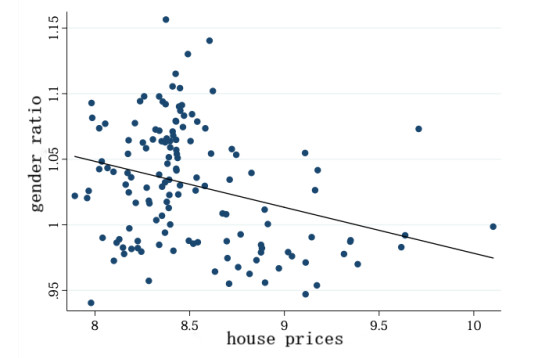
We investigated the relationship between changes in housing prices and marriage patterns among Chinese residents, considering the evolving real estate market and increasing prevalence of homogamous marriages. Using microdata from the China Household Income Project (CHIP) and urban housing price data, our results showed the following: First, housing price levels significantly decreased the likelihood of residents engaging in hypergamous mating and marrying individuals from lower social strata. Second, regional fluctuations in housing prices could influence residents' marital matches by affecting the spatial distribution of genders. Specifically, the higher the level of urban house prices, the greater the crowding out effect on marriageable men, and the less likely men in that area were to match downwards and marry women from lower social classes. Third, heterogeneity analysis indicated that residents in the eastern regions, younger populations, and migrants faced greater housing price pressures in the process of marital matching, resulting in a more substantial impact on these groups. The study contributes to marriage matching theories and offers policy insights for real estate reforms.
Citation: Jiajia He, Xiuping Zou, Tinghui Li. House price, gender spatial allocation, and the change of marriage matching[J]. AIMS Mathematics, 2024, 9(4): 8079-8103. doi: 10.3934/math.2024393
We investigated the relationship between changes in housing prices and marriage patterns among Chinese residents, considering the evolving real estate market and increasing prevalence of homogamous marriages. Using microdata from the China Household Income Project (CHIP) and urban housing price data, our results showed the following: First, housing price levels significantly decreased the likelihood of residents engaging in hypergamous mating and marrying individuals from lower social strata. Second, regional fluctuations in housing prices could influence residents' marital matches by affecting the spatial distribution of genders. Specifically, the higher the level of urban house prices, the greater the crowding out effect on marriageable men, and the less likely men in that area were to match downwards and marry women from lower social classes. Third, heterogeneity analysis indicated that residents in the eastern regions, younger populations, and migrants faced greater housing price pressures in the process of marital matching, resulting in a more substantial impact on these groups. The study contributes to marriage matching theories and offers policy insights for real estate reforms.

| [1] |
H. Han, Trends in educational assortative marriage in China from 1970 to 2000, Demographic Res., 22 (2010), 733–770. https://doi.org/10.4054/DemRes.2010.22.24 doi: 10.4054/DemRes.2010.22.24

|
| [2] |
J. Smits, H. Park, Five decades of educational assortative mating in 10 East Asian societies, Soc. Forces, 88 (2009), 227–255. https://doi.org/10.1353/sof.0.0241 doi: 10.1353/sof.0.0241
|
| [3] |
X. Xu, J. Ji, Y. Y. Tung, Social and political assortative mating in urban China, J. Fam. Issues, 21 (2000), 47–77. https://doi.org/10.1177/019251300021001003 doi: 10.1177/019251300021001003
|
| [4] |
Z. Mu, Y. Xie, Marital age homogamy in China: a reversal of trend in the reform era, Soc. Sci. Res., 44 (2014), 141–157. https://doi.org/10.1016/j.ssresearch.2013.11.005 doi: 10.1016/j.ssresearch.2013.11.005
|
| [5] |
K. K. Charles, E. Hurst, A. Killewald, Marital sorting and parental wealth, Demography, 50 (2012), 51–70. https://doi.org/10.1007/s13524-012-0144-6 doi: 10.1007/s13524-012-0144-6
|
| [6] |
A. J. Plantinga, C. Détang-Dessendre, G. L. Hunt, V. Piguet, Housing prices and inter-urban migration, Reg. Sci. Urban Econ., 43 (2013), 296–306. https://doi.org/10.1016/j.regsciurbeco.2012.07.009 doi: 10.1016/j.regsciurbeco.2012.07.009
|
| [7] |
J. Graham, C. A. Makridis, House prices and consumption: a new instrumental variables approach, Amer. Econ. J.: Macroecon., 15 (2023), 411–443. https://doi.org/10.1257/mac.20200246 doi: 10.1257/mac.20200246
|
| [8] |
C. W. Peng, I. C. Tsai, The long- and short-run influences of housing prices on migration, Cities. 93 (2019), 253–262. https://doi.org/10.1016/j.cities.2019.05.011 doi: 10.1016/j.cities.2019.05.011
|
| [9] |
L. J. Dettling, M. S. Kearney, House prices and birth rates: the impact of the real estate market on the decision to have a baby, J. Public Econ., 110 (2014), 82–100. https://doi.org/10.1016/j.jpubeco.2013.09.009 doi: 10.1016/j.jpubeco.2013.09.009
|
| [10] |
G. S. Becker, A theory of marriage: part Ⅰ, J. Politic. Econ., 81 (1973), 813–846. https://doi.org/10.1086/260084 doi: 10.1086/260084
|
| [11] | G. S. Becker, A theory of marriage: part Ⅱ, J. Political Econ., 82 (1973), S11–S26. |
| [12] |
S. Sargeson, Subduing "The rural house-building craze": attitudes towards housing construction and land use controls in four Zhejiang villages, China Quart., 172 (2002), 927–955. https://doi.org/10.1017/S0009443902000566 doi: 10.1017/S0009443902000566
|
| [13] |
J. M. Raymo, Y. Xie, Temporal and regional variation in the strength of educational homogamy, Amer. Sociol. Rev., 65 (2000), 773–781. https://doi.org/10.1177/000312240006500508 doi: 10.1177/000312240006500508
|
| [14] |
D. H. Wrenn, J. Yi, B. Zhang, House prices and marriage entry in China, Reg. Sci. Urban Econ., 74 (2019), 118–130. https://doi.org/10.1016/j.regsciurbeco.2018.12.001 doi: 10.1016/j.regsciurbeco.2018.12.001
|
| [15] |
M. Farnham, L. Schmidt, P. Sevak, House prices and marital stability, Amer. Econ. Rew., 101 (2011), 615–619. https://doi.org/10.1257/aer.101.3.615 doi: 10.1257/aer.101.3.615
|
| [16] |
D. Lam, Marriage markets and assortative mating with household public goods: theoretical results and empirical implications, J. Hum. Resour., 23 (1988), 462–487. https://doi.org/10.2307/145809 doi: 10.2307/145809
|
| [17] |
K. Basu, Gender and say: a model of household behaviour with endogenously determined balance of power, Econ. J., 116 (2006), 558–580. https://doi.org/10.1111/j.1468-0297.2006.01092.x doi: 10.1111/j.1468-0297.2006.01092.x
|
| [18] |
A. Sun, Q. Zhang, Who marries whom in a surging housing market, J. Dev. Econ., 146 (2020), 102492. https://doi.org/10.1016/j.jdeveco.2020.102492 doi: 10.1016/j.jdeveco.2020.102492
|
| [19] |
D. Gray, Housing market activity diffusion in England and Wales, Natl. Account. Rev., 5 (2023), 125–144. https://doi.org/10.3934/NAR.2023008 doi: 10.3934/NAR.2023008
|
| [20] |
Z. Li, J. Zhong, Impact of economic policy uncertainty shocks on China's financial conditions, Financ. Res. Lett., 35 (2020), 101303. https://doi.org/10.1016/j.frl.2019.101303 doi: 10.1016/j.frl.2019.101303
|
| [21] |
Z. Li, C. Yang, Z. Huang, How does the fintech sector react to signals from central bank digital currencies, Financ. Res. Lett., 50 (2022), 103308. https://doi.org/10.1016/j.frl.2022.103308 doi: 10.1016/j.frl.2022.103308
|
| [22] |
Z. Dong, E. C. M. Hui, S. Jia, How does housing price affect consumption in China: wealth effect or substitution effect, Cities, 64 (2017), 1–8. https://doi.org/10.1016/j.cities.2017.01.006 doi: 10.1016/j.cities.2017.01.006
|
| [23] |
T. C. Chiang, Stock returns and inflation expectations: evidence from 20 major countries, Quant. Financ. Econ., 7 (2023), 538–568. https://doi.org/10.3934/QFE.2023027 doi: 10.3934/QFE.2023027
|
| [24] |
R. Abramitzky, A. Delavande, L. Vasconcelos, Marrying up: the role of sex ratio in assortative matching, Amer. Econ. J.: Appl. Econ., 3 (2011), 124–157. https://doi.org/10.1257/app.3.3.124 doi: 10.1257/app.3.3.124
|
| [25] | G. S. Becker, A treatise on the family, Harvard University Press, 1991. https://doi.org/10.2307/j.ctv322v4rc |
| [26] |
X. Lei, J. P. Smith, X. Sun, Y. Zhao, Gender differences in cognition in China and reasons for change over time: evidence from CHARLS, J. Econ. Ageing, 4 (2014), 46–55. https://doi.org/10.1016/j.jeoa.2013.11.001 doi: 10.1016/j.jeoa.2013.11.001
|
| [27] |
J. F. Hair, J. J. García-Machado, M. Martínez-Avila, The impact of organizational compliance culture and green culture on environmental behavior: the moderating effect of environmental commitment, Green Financ., 5 (2023), 624–657. https://doi.org/10.3934/GF.2023024 doi: 10.3934/GF.2023024
|
| [28] |
J. Liu, C. Xing, Q. Zhang, House price, fertility rates and reproductive intentions, China Econ. Rev., 62 (2020), 101496. https://doi.org/10.1016/j.chieco.2020.101496 doi: 10.1016/j.chieco.2020.101496
|
| [29] |
A. Grossbard-Shechtman, Economic behavior, marriage and fertility: two lessons from polygyny, J. Econ. Behavior Organ., 7 (1986), 415–424. https://doi.org/10.1016/0167-2681(86)90014-4 doi: 10.1016/0167-2681(86)90014-4
|
| [30] | S. Grossbard, A theory of allocation of time in markets for labor and marriage: macromodel, In: S. Grossbard, The marriage motive: a price theory of marriage: how marriage markets affect employment, consumption, and savings, New York: Springer, 2015, 21–32. https://doi.org/10.1007/978-1-4614-1623-4_2 |
| [31] |
J. Du, Y. Wang, Y. Zhang, Sex imbalance, marital matching and intra-household bargaining: evidence from China, China Econ. Rev., 35 (2015), 197–218. https://doi.org/10.1016/j.chieco.2014.11.002 doi: 10.1016/j.chieco.2014.11.002
|
| [32] |
M. Porter, How do sex ratios in China influence marriage decisions and intra-household resource allocation, Rev. Econ. Household., 14 (2016), 337–371. https://doi.org/10.1007/s11150-014-9262-9 doi: 10.1007/s11150-014-9262-9
|
| [33] |
Z. Li, Z. Huang, Y. Su, New media environment, environmental regulation and corporate green technology innovation: evidence from China, Energy Econ., 119 (2023), 106545. https://doi.org/10.1016/j.eneco.2023.106545 doi: 10.1016/j.eneco.2023.106545
|
| [34] |
C. Zheng, M. A. M. Khan, M. M. Rahman, S. B. Sadeque, R. Islam, The impact of monetary policy on banks' risk-taking behavior in an emerging economy: the role of basel Ⅱ, Data Sci. Financ. Econ., 3 (2023), 427–451. https://doi.org/10.3934/DSFE.2023024 doi: 10.3934/DSFE.2023024
|
| [35] |
Z. Li, B. Mo, H. Nie, Time and frequency dynamic connectedness between cryptocurrencies and financial assets in China, Int. Rev. Econ. Financ., 86 (2023), 46–57. https://doi.org/10.1016/j.iref.2023.01.015 doi: 10.1016/j.iref.2023.01.015
|
| [36] |
Y. Wen, Y. Xu, Statistical monitoring of economic growth momentum transformation: empirical study of Chinese provinces, AIMS Math., 8 (2023), 24825–24847. https://doi.org/10.3934/math.20231266 doi: 10.3934/math.20231266
|
| [37] |
M. Hong, J. He, K. Zhang, Z. Guo, Does digital transformation of enterprises help reduce the cost of equity capital, Math. Biosci. Eng., 20 (2023), 6498–6516. https://doi.org/10.3934/mbe.2023280 doi: 10.3934/mbe.2023280
|
| [38] |
Y. Liu, Z. Li, M. Xu, The influential factors of financial cycle spillover: evidence from China, Emerg. Mark. Financ. Trade, 56 (2020), 1336–1350. https://doi.org/10.1080/1540496X.2019.1658076 doi: 10.1080/1540496X.2019.1658076
|
| [39] |
Y. Liu, Y. Wen, Y. Xiao, L. Zhang, S. Huang, Identification of the enterprise financialization motivation on crowding out R&D innovation: evidence from listed companies in China, AIMS Math., 9 (2024), 5951–5970. https://doi.org/10.3934/math.2024291 doi: 10.3934/math.2024291
|
| [40] |
Y. Liu, L. Chen, H. Luo, Y. Liu, Y. Wen, The impact of intellectual property rights protection on green innovation: a quasi-natural experiment based on the pilot policy of the Chinese intellectual property court, Math. Biosci. Eng., 21 (2024), 2587–2607. https://doi.org/10.3934/mbe.2024114 doi: 10.3934/mbe.2024114
|
| [41] |
V. Hlasny, Social assistance and workers' long-term well-being in Egypt, Natl. Account. Rev., 5 (2023), 174–185. https://doi.org/10.3934/NAR.2023011 doi: 10.3934/NAR.2023011
|
| [42] |
Y. Lin, X. Chen, H. Lan, Analysis and prediction of American economy under different government policy based on stepwise regression and support vector machine modelling, Data Sci. Financ. Econ., 3 (2023), 1–13. https://doi.org/10.3934/DSFE.2023001 doi: 10.3934/DSFE.2023001
|
| [43] |
Z. Li, H. Dong, C. Floros, A. Charemis, P. Failler, Re-examining Bitcoin volatility: a CAViaR-based approach, Emerg. Mark. Financ. Trade, 58 (2022), 1320–1338. https://doi.org/10.1080/1540496X.2021.1873127 doi: 10.1080/1540496X.2021.1873127
|
| [44] | Z. Li, L. Chen, H. Dong, What are bitcoin market reactions to its-related events, Int. Rev. Econ. Financ., 73 (2021), 1–10. |
| [45] |
Z. Li, H. Chen, B. Mo, Can digital finance promote urban innovation? Evidence from China, Borsa Istanbul Rev., 23 (2023), 285–296. https://doi.org/10.1016/j.bir.2022.10.006 doi: 10.1016/j.bir.2022.10.006
|
| [46] |
G. Liu, H. Yi, H. Liang, Measuring provincial digital finance development efficiency based on stochastic frontier model, Quant. Financ. Econ., 7 (2023), 420–439. https://doi.org/10.3934/QFE.2023021 doi: 10.3934/QFE.2023021
|
| [47] |
S. L. N. Alonso, Can Central Bank Digital Currencies be green and sustainable, Green Financ., 5 (2023), 603–623. https://doi.org/10.3934/GF.2023023 doi: 10.3934/GF.2023023
|
| [48] |
Z. Li, J. Zhu, J. He, The effects of digital financial inclusion on innovation and entrepreneurship: a network perspective, Electron. Res. Arch., 30 (2022), 4697–4715. https://doi.org/10.3934/era.2022238 doi: 10.3934/era.2022238
|


Figures(3) / Tables(8)

Jiajia He, Xiuping Zou, Tinghui Li. House price, gender spatial allocation, and the change of marriage matching[J]. AIMS Mathematics, 2024, 9(4): 8079-8103. doi: 10.3934/math.2024393


 DownLoad: