Dynamic analysis and optimum control of a rumor spreading model with multivariate gatekeepers

Yanchao Liu; Pengzhou Zhang; Deyu Li; Junpeng Gong; Yanchao Liu; Pengzhou Zhang; Deyu Li; Junpeng Gong

doi:10.3934/math.20241522

AIMS Mathematics

2024, Volume 9, Issue 11: 31658-31678. doi: 10.3934/math.20241522

Previous Article Next Article

Research article

Dynamic analysis and optimum control of a rumor spreading model with multivariate gatekeepers

State Key Laboratory of Media Convergence and Communication, Communication University of China, No.1 Dingfuzhuang East Street, Chaoyang District, Beijing 100024, China

Received: 16 September 2024 Revised: 17 October 2024 Accepted: 24 October 2024 Published: 07 November 2024
MSC : 34D23, 49J15

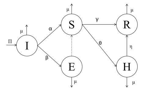
Rumor spreading on social media platforms can significantly impact public opinion and decision-making. In this paper, we proposed an innovative ignorant-spreader-expositor-hibernator-remover (ISEHR) rumor-spreading model with multivariate gatekeepers. Specifically, by analyzing the model's dynamics, we identified the critical threshold that determined the persistence or extinction of rumor spreading. Moreover, we applied the Routh-Hurwitz judgment, Lyapunov theory, and LaSalle's invariance principle to investigate the existence and stability of the rumor-free/rumor equilibrium points. Furthermore, we introduced the optimal control to alleviate rumor spreading with the multivariate gatekeeper mechanism. Finally, extensive numerical simulations validated our theoretical findings, providing insights into the complex dynamics of rumor spreading and the effectiveness of the proposed control measures. Our research contributes to a deeper understanding of rumor spreading on social networks, offering valuable implications for the development of effective strategies to combat rumor.

Keywords:

Citation: Yanchao Liu, Pengzhou Zhang, Deyu Li, Junpeng Gong. Dynamic analysis and optimum control of a rumor spreading model with multivariate gatekeepers[J]. AIMS Mathematics, 2024, 9(11): 31658-31678. doi: 10.3934/math.20241522

Related Papers:

[1]	Meshari Alesemi . Innovative approaches of a time-fractional system of Boussinesq equations within a Mohand transform. AIMS Mathematics, 2024, 9(10): 29269-29295. doi: 10.3934/math.20241419
[2]	Azzh Saad Alshehry, Humaira Yasmin, Ali M. Mahnashi . Exploring fractional Advection-Dispersion equations with computational methods: Caputo operator and Mohand techniques. AIMS Mathematics, 2025, 10(1): 234-269. doi: 10.3934/math.2025012
[3]	Shabir Ahmad, Aman Ullah, Ali Akgül, Fahd Jarad . A hybrid analytical technique for solving nonlinear fractional order PDEs of power law kernel: Application to KdV and Fornberg-Witham equations. AIMS Mathematics, 2022, 7(5): 9389-9404. doi: 10.3934/math.2022521
[4]	Abdul Samad, Imran Siddique, Fahd Jarad . Meshfree numerical integration for some challenging multi-term fractional order PDEs. AIMS Mathematics, 2022, 7(8): 14249-14269. doi: 10.3934/math.2022785
[5]	Mamta Kapoor, Nehad Ali Shah, Wajaree Weera . Analytical solution of time-fractional Schrödinger equations via Shehu Adomian Decomposition Method. AIMS Mathematics, 2022, 7(10): 19562-19596. doi: 10.3934/math.20221074
[6]	Abdul Samad, Imran Siddique, Zareen A. Khan . Meshfree numerical approach for some time-space dependent order partial differential equations in porous media. AIMS Mathematics, 2023, 8(6): 13162-13180. doi: 10.3934/math.2023665
[7]	M. S. Alqurashi, Saima Rashid, Bushra Kanwal, Fahd Jarad, S. K. Elagan . A novel formulation of the fuzzy hybrid transform for dealing nonlinear partial differential equations via fuzzy fractional derivative involving general order. AIMS Mathematics, 2022, 7(8): 14946-14974. doi: 10.3934/math.2022819
[8]	Asif Khan, Tayyaba Akram, Arshad Khan, Shabir Ahmad, Kamsing Nonlaopon . Investigation of time fractional nonlinear KdV-Burgers equation under fractional operators with nonsingular kernels. AIMS Mathematics, 2023, 8(1): 1251-1268. doi: 10.3934/math.2023063
[9]	Muhammad Imran Liaqat, Sina Etemad, Shahram Rezapour, Choonkil Park . A novel analytical Aboodh residual power series method for solving linear and nonlinear time-fractional partial differential equations with variable coefficients. AIMS Mathematics, 2022, 7(9): 16917-16948. doi: 10.3934/math.2022929
[10]	Aliaa Burqan, Mohammed Shqair, Ahmad El-Ajou, Sherif M. E. Ismaeel, Zeyad AlZhour . Analytical solutions to the coupled fractional neutron diffusion equations with delayed neutrons system using Laplace transform method. AIMS Mathematics, 2023, 8(8): 19297-19312. doi: 10.3934/math.2023984

Abstract

1. Introduction

Mathematical methods have been used to represent a variety of real-world issues. For example, we can approximate a body's speed for a given distance and time by using the concept of rate of change. Specifically, we use the notion of differential calculus. Many complicated phenomena, such as chaos, solitons, asymptotic properties, singular formation, and others, are either poorly projected or have not yet been discovered ^[1,2,3]. Furthermore, the notion of calculus with differential operators and integrals is essential for describing physical phenomena and divining natural events connected to variation and changes. However, while researching issues with hereditary characteristics or memory, numerous researchers found numerous shortcomings and restrictions in integer-order calculus ^[4,5]. Later, new operators defined with the aid of fractional-order were proposed by mathematicians and physicists. Many researchers are drawn to fractional calculus (FC) while looking at different models ^[6,7,8].

In many branches of physical science and engineering, fractional calculus, which deals with arbitrary order derivatives and integrals, is crucial ^[9]. Fractional calculus and its applications have developed rapidly in the last few years ^[10,11]. Significant issues in acoustics, fluid mechanics, electromagnetic, analytical chemistry, signal processing, biology, and many other engineering and physical science branches are modeled by nonlinear and linear partial differential equations (PDEs) ^[12]. Both nonlinear and linear FDEs have been solved analytically and numerically in recent years using a variety of techniques, including the Yang-Laplace transform ^[13], the Adomian decomposition method ^[14], the homotopy analysis method ^[15], and the Laplace decomposition method ^[16]. Furthermore, nonlinear and linear FDEs are also subjected to the local fractional variational iteration approach ^[17,18], the fractional complex transform method ^[19], the modified Laplace decomposition approach ^[16,20], and the cylindrical-coordinate method ^[21].

Mathematical models known as fractional partial differential equations (FPDEs) depict physical processes that exhibit complicated dynamics and non-local effects. FPDEs represent an expansion of the traditional theory of partial differential equations. They enable non-integer orders of differentiation, which more accurately capture the non-local and nonlinear characteristics of an extensive range of physical systems ^[22,23]. These formulas are being used more and more frequently in several fields, such as biology, engineering, economics, and physics. These formulas are valuable resources for constructing intricate systems and examining the behavior of those operations. This article explores the concept of fractional-order partial differential equations, their applications, and the challenges associated with their analysis and numerical solution ^[24,25,26].

In 2013, Al-Smadi proposed the Residual Power Series Method (RPSM) ^[27]. It is generated from the residual error function mixed with the Taylor series. The solution to the problem is an infinite convergence series ^[28,29,30]. Many DEs have inspired fresh RPSM algorithms ^[31,32,33]. Among these DEs are several Boussinesq DEs, fuzzy DEs, and KdV Burger's equation, among many others. These systems are built to generate exact and efficient approximations. We provide a technique to investigate the approximation of solutions to fractional PDEs and systems of PDEs using RPSM in the Mohand transform (MT) formulation. The computational series finds the exact solution after a few iterations ^{[34,35,36,37]}.

The computational complexity and effort necessary to implement the methods that were previously discussed are among the most significant constraints. The Mohand distinguishes our work transform iterative methodology (MTIM), which we developed as an iterative approach to addressing fractional PDEs and systems of PDEs. This technique is highly effective in reducing the amount of computational work and complexity necessary due to integrating the MT with the new iterative process.

In this study, the Mohand residual power series method (MRPSM) and MTIM are used to solve fractional PDEs and systems of PDEs. The numerical values produced by these techniques are more precise when compared to those of other numerical procedures. This study includes a comparison study of the numerical data. A strong indicator of the efficacy and reliability of these methods is the fact that the results of the many approaches presented are compatible with one another. The attractiveness of fractional-order derivatives grows in direct correlation with their worth. Because of this, the algorithms can withstand spikes in computational error, are easy to use, and are quick and accurate. Discovering this will make solving many partial differential equations much easier for mathematicians.

2. Mohand transformation

The portions that follow will cover the basic elements and ideas of the MT, providing the foundation for this operation.

Definition 2.1. The MT of the function $\mathfrak{P}(\mathfrak{t})$ is defined as ^[38]

$M[\mathfrak{P}(\mathfrak{t})] = R(s) = s^2\displaystyle{\int}_{0}^{\mathfrak{t}}\mathfrak{P}(\mathfrak{t})e^{-s\mathfrak{t}}d{\mathfrak{t}},\ \ {k}_{1}\leq s \leq{k}_{2}.$

The inverse Mohand transform (IMT) is defined as

$M^{-1}[R(s)] = \mathfrak{P}(\mathfrak{t}).$

Definition 2.2. (^[39]). The derivative of fractional-order in the framework of MT is defined as

$M[\mathfrak{P}^{\mathfrak{F}}(\mathfrak{t})] = s^{\mathfrak{F}}R(s)-\sum\limits_{k = 0}^{n-1}\frac{\mathfrak{P}^{k}(0)}{s^{k-(\mathfrak{F}+1)}},\ 0 < \mathfrak{F}\leq n.$

Definition 2.3. The properties of MT are given as follows:

(1) $M[\mathfrak{P}'(\mathfrak{t})] = sR(s)-s^{2}R(0)$ .

(2) $M[\mathfrak{P}''(\mathfrak{t})] = s^{2}R(s)-s^{3}R(0)-s^{2}R'(0)$ .

(3) $M[\mathfrak{P}^{n}(\mathfrak{t})] = s^{n}R(s)-s^{n+1}R(0)-s^{n}R'(0)-\cdots-s^{n}R^{n-1}(0)$ .

Lemma 2.4. Suppose there exists a function represented by $\mathfrak{P}({{\mathfrak{R}}}, {{\mathfrak{t}}})$ , having exponential order. $M[R(s)] = \mathfrak{P}({{\mathfrak{R}}}, {{\mathfrak{t}}})$ denotes the MT in this case:

$\begin{equation} M[D_{{{\mathfrak{t}}}}^{r{\mathfrak{F}}}\mathfrak{P}({{\mathfrak{R}}}, {{\mathfrak{t}}})] = {s}^{r{\mathfrak{F}}}R(s)-\sum\limits_{j = 0}^{r-1}{s}^{{\mathfrak{F}}(r-j)-1}D_{{{\mathfrak{t}}}}^{j{\mathfrak{F}}}\mathfrak{P}({{\mathfrak{R}}},0), 0 < {\mathfrak{F}}\leq 1, \end{equation}$

(2.1)

where ${{\mathfrak{R}}} = ({{\mathfrak{R}}}_{1}, {{\mathfrak{R}}}_{2}, \cdots, {{\mathfrak{R}}}_{\mathfrak{F}})\in \mathbb{R}^{\mathfrak{F}}$ , $\mathfrak{F}\in \mathbb{N}$ , and $D_{{{\mathfrak{t}}}}^{r{\mathfrak{F}}} = D_{{{\mathfrak{t}}}}^{{\mathfrak{F}}}.D_{{{\mathfrak{t}}}}^{{\mathfrak{F}}}.\cdots.D_{{{\mathfrak{t}}}}^{{\mathfrak{F}}}(r-times)$ .

Proof. To validate Eq (2.4), we use the induction method. Taking $r = 1$ in Eq (2.4):

$M[D_{{{\mathfrak{t}}}}^{2{\mathfrak{F}}}\mathfrak{P}({{\mathfrak{R}}}, {{\mathfrak{t}}})] = {s}^{2{\mathfrak{F}}}R(s)-{s}^{2{\mathfrak{F}}-1}\mathfrak{P}({{\mathfrak{R}}},0)-{s}^{{\mathfrak{F}}-1}D_{{{\mathfrak{t}}}}^{{\mathfrak{F}}}\mathfrak{P}({{\mathfrak{R}}},0).$

Equation (2.4) is true for $r = 1$ on the basis of Definition 2.2. Now, put $r = 2$ in Eq (2.4) to obtain the following outcome:

$\begin{equation} M[D_{r}^{2{\mathfrak{F}}}\mathfrak{P}({{\mathfrak{R}}}, {{\mathfrak{t}}})] = {s}^{2{\mathfrak{F}}}R(s)-{s}^{2{\mathfrak{F}}-1}\mathfrak{P}({{\mathfrak{R}}},0)-{s}^{{\mathfrak{F}}-1}D_{{{\mathfrak{t}}}}^{{\mathfrak{F}}}\mathfrak{P}({{\mathfrak{R}}},0). \end{equation}$

(2.2)

We obtain the next result from the LHS of Eq (2.2):

$\begin{equation} L.H.S = M[D_{{{\mathfrak{t}}}}^{2{\mathfrak{F}}}\mathfrak{P}({{\mathfrak{R}}}, {{\mathfrak{t}}})]. \end{equation}$

(2.3)

We may also write Eq (2.3) as

$\begin{equation} L.H.S = M[D_{{{\mathfrak{t}}}}^{{\mathfrak{F}}}D_{{{\mathfrak{t}}}}^{{\mathfrak{F}}}\mathfrak{P}({{\mathfrak{R}}}, {{\mathfrak{t}}})]. \end{equation}$

(2.4)

Assume

$\begin{equation} z({{\mathfrak{R}}}, {{\mathfrak{t}}}) = D_{{{\mathfrak{t}}}}^{{\mathfrak{F}}}\mathfrak{P}({{\mathfrak{R}}}, {{\mathfrak{t}}}). \end{equation}$

(2.5)

Putting Eq (2.5) in Eq (2.4),

$\begin{equation} L.H.S = M[D_{{{\mathfrak{t}}}}^{{\mathfrak{F}}}z({{\mathfrak{R}}}, {{\mathfrak{t}}})]. \end{equation}$

(2.6)

Using the derivative of Caputo, Eq (2.6) becomes

$\begin{equation} L.H.S = M[J^{1-{\mathfrak{F}}}z^{'}({{\mathfrak{R}}}, {{\mathfrak{t}}})]. \end{equation}$

(2.7)

Applying the RL integral on Eq (2.7),

$\begin{equation} L.H.S = \frac{M[z^{'}({{\mathfrak{R}}}, {{\mathfrak{t}}})]}{{s}^{1-{\mathfrak{F}}}}. \end{equation}$

(2.8)

The derivative property of MT is applied on Eq (2.8) to obtain the following result:

$\begin{equation} L.H.S = {s}^{{\mathfrak{F}}}Z({{\mathfrak{R}}},{s})-\frac{z({{\mathfrak{R}}},0)}{{s}^{1-{\mathfrak{F}}}}. \end{equation}$

(2.9)

Using Eq (2.5), we obtain

$Z({{\mathfrak{R}}},{s}) = {s}^{{\mathfrak{F}}}R(s)-\frac{\mathfrak{P}({{\mathfrak{R}}},0)}{{s}^{1-{\mathfrak{F}}}}.$

As $M[z({{\mathfrak{t}}}, {{\mathfrak{R}}})] = Z({{\mathfrak{R}}}, {s})$ , we can write Eq (2.9) as

$\begin{equation} L.H.S = {s}^{2{\mathfrak{F}}}R(s)-\frac{\mathfrak{P}({{\mathfrak{R}}},0)}{{s}^{1-2{\mathfrak{F}}}}-\frac{D_{{{\mathfrak{t}}}}^{{\mathfrak{F}}}\mathfrak{P}({{\mathfrak{R}}},0)}{{s}^{1-{\mathfrak{F}}}}. \end{equation}$

(2.10)

Assume that Eq (2.4) is true for $r = K$ . Taking $r = K$ in Eq (2.4),

$\begin{equation} M[D_{{{\mathfrak{t}}}}^{K{\mathfrak{F}}}\mathfrak{P}({{\mathfrak{R}}}, {{\mathfrak{t}}})] = {s}^{K{\mathfrak{F}}}R(s)-\sum\limits_{j = 0}^{K-1}{s}^{{\mathfrak{F}}(K-j)-1}D_{{{\mathfrak{t}}}}^{j{\mathfrak{F}}}D_{{{\mathfrak{t}}}}^{j{\mathfrak{F}}}\mathfrak{P}({{\mathfrak{R}}},0),\ 0 < {\mathfrak{F}}\leq1. \end{equation}$

(2.11)

Next, we will have to show that Eq (2.4) for $r = K+1$ holds. Taking $r = K+1$ in Eq (2.4),

$\begin{equation} M[D_{{{\mathfrak{t}}}}^{(K+1){\mathfrak{F}}}\mathfrak{P}({{\mathfrak{R}}}, {{\mathfrak{t}}})] = {s}^{(K+1){\mathfrak{F}}}R(s)-\sum\limits_{j = 0}^{K}{s}^{{\mathfrak{F}}((K+1)-j)-1}D_{{{\mathfrak{t}}}}^{j{\mathfrak{F}}}\mathfrak{P}({{\mathfrak{R}}},0). \end{equation}$

(2.12)

From the left-hand side of Eq (2.12), we derive

$\begin{equation} L.H.S = M[D_{{{\mathfrak{t}}}}^{K{\mathfrak{F}}}(D_{{{\mathfrak{t}}}}^{K{\mathfrak{F}}})]. \end{equation}$

(2.13)

Letting $D_{{{\mathfrak{t}}}}^{K{\mathfrak{F}}} = g({{\mathfrak{R}}}, {{\mathfrak{t}}}),$ Eq (2.13) gives us

$\begin{equation} L.H.S = M[D_{{{\mathfrak{t}}}}^{{\mathfrak{F}}}g({{\mathfrak{R}}}, {{\mathfrak{t}}})]. \end{equation}$

(2.14)

Applying Caputo's derivative and the RL integral on Eq (2.14),

$\begin{equation} L.H.S = {s}^{{\mathfrak{F}}}M[D_{{{\mathfrak{t}}}}^{K{\mathfrak{F}}}\mathfrak{P}({{\mathfrak{R}}}, {{\mathfrak{t}}})]-\frac{g({{\mathfrak{R}}},0)}{{s}^{1-{\mathfrak{F}}}}. \end{equation}$

(2.15)

On the basis of Eq (2.11), we can write Eq (2.15) as

$\begin{equation} L.H.S = {s}^{r{\mathfrak{F}}}R(s)-\sum\limits_{j = 0}^{r-1}{s}^{{\mathfrak{F}}(r-j)-1}D_{{{\mathfrak{t}}}}^{j{\mathfrak{F}}}\mathfrak{P}({{\mathfrak{R}}},0). \end{equation}$

(2.16)

Equation (2.16) can also be written as

$L.H.S = M[D_{{{\mathfrak{t}}}}^{r{\mathfrak{F}}}\mathfrak{P}({{\mathfrak{R}}},0)].$

Using mathematical induction, Eq (2.4) is true for $r = K+1$ . Hence, it is proved that for all positive integers, Eq (2.4) holds. □

Lemma 2.5. Let assume that there exists an exponential-order function $\mathfrak{P}({{\mathfrak{R}}}, {{\mathfrak{t}}})$ . $M[\mathfrak{P}({{\mathfrak{R}}}, {{\mathfrak{t}}})] = R(s)$ denotes the MT of $\mathfrak{P}({{\mathfrak{R}}}, {{\mathfrak{t}}})$ . The multiple fractional power series (MFPS) in MT is given as

$\begin{equation} R(s) = \sum\limits_{r = 0}^{\infty}\frac{\hbar_{r}({{\mathfrak{R}}})}{s^{r{\mathfrak{F}}+1}}, s > 0, \end{equation}$

(2.17)

where, ${{\mathfrak{R}}} = (s_{1}, {{\mathfrak{R}}}_{2}, \cdots, {{\mathfrak{R}}}_{\mathfrak{F}})\in\mathbb{R}^{\mathfrak{F}}, \ \mathfrak{F}\in \mathbb{N}$ .

Proof. Let us consider the Taylor series

$\begin{equation} \mathfrak{P}({{\mathfrak{R}}}, {{\mathfrak{t}}}) = \hbar_{0}({{\mathfrak{R}}})+\hbar_{1}({{\mathfrak{R}}})\frac{{{\mathfrak{t}}}^{{\mathfrak{F}}}}{\Gamma[{\mathfrak{F}}+1]}++\hbar_{2}({{\mathfrak{R}}})\frac{{{\mathfrak{t}}}^{2{\mathfrak{F}}}}{\Gamma[2{\mathfrak{F}}+1]}+\cdots. \end{equation}$

(2.18)

MT is subjected to Eq (2.18) to obtain

$M\left[\mathfrak{P}({{\mathfrak{R}}}, {{\mathfrak{t}}})\right] = M\left[\hbar_{0}({{\mathfrak{R}}})\right]+M\left[\hbar_{1}({{\mathfrak{R}}})\frac{{{\mathfrak{t}}}^{{\mathfrak{F}}}}{\Gamma[{\mathfrak{F}}+1]}\right]+M\left[\hbar_{1}({{\mathfrak{R}}}) \frac{{{\mathfrak{t}}}^{2{\mathfrak{F}}}}{\Gamma[2{\mathfrak{F}}+1]}\right]+\cdots.$

Utilizing the features of MT, we derive

$M\left[\mathfrak{P}({{\mathfrak{R}}}, {{\mathfrak{t}}})\right] = \hbar_{0}({{\mathfrak{R}}})\frac{1}{s}+\hbar_{1}({{\mathfrak{R}}})\frac{\Gamma[{\mathfrak{F}}+1]}{\Gamma[{\mathfrak{F}}+1]}\frac{1}{s^{{\mathfrak{F}}+1}}+\hbar_{2}({{\mathfrak{R}}}) \frac{\Gamma[2{\mathfrak{F}}+1]}{\Gamma[2{\mathfrak{F}}+1]}\frac{1}{s^{2{\mathfrak{F}}+1}}\cdots.$

Thus, a new Taylor series form is obtained. □

Lemma 2.6. If $M[\mathfrak{P}(\mathfrak{R}, \mathfrak{t})] = R(s)$ denotes MT, then the new Taylor series form in MFPS is given as

$\begin{equation} \hbar_{0}({{\mathfrak{R}}}) = \lim\limits_{s\rightarrow \infty}sR(s) = \mathfrak{P}({{\mathfrak{R}}},0). \end{equation}$

(2.19)

Proof. Assume the Taylor's series

$\begin{equation} \hbar_{0}({{\mathfrak{R}}}) = sR(s)-\frac{\hbar_{1}({{\mathfrak{R}}})}{s^{{\mathfrak{F}}}}-\frac{\hbar_{2}({{\mathfrak{R}}})}{s^{2{\mathfrak{F}}}}-\cdots. \end{equation}$

(2.20)

When the limit in Eq (2.19) is calculated and simplified, we get Eq (2.20). □

3. Mohand residual power series method

In this part, we construct the framework of the proposed method for the solution of fractional PDEs.

Step 1. Let us assume the fractional PDE

$\begin{equation} D_{{{\mathfrak{t}}}}^{{\mathfrak{F}}}\mathfrak{P}({{\mathfrak{R}}}, {{\mathfrak{t}}})+\mathfrak{K}({{\mathfrak{R}}})N(\mathfrak{P})-\delta({{\mathfrak{R}}},\mathfrak{P}) = 0. \end{equation}$

(3.1)

Step 2. Applying the MT on both sides of Eq (3.1),

$\begin{equation} M[D_{{{\mathfrak{t}}}}^{{\mathfrak{F}}}\mathfrak{P}({{\mathfrak{R}}}, {{\mathfrak{t}}})+\mathfrak{K}({{\mathfrak{R}}})N(\mathfrak{P})-\delta({{\mathfrak{R}}},\mathfrak{P})] = 0. \end{equation}$

(3.2)

On the basis of Lemma 2.4, we derive

$\begin{equation} R(s) = \sum\limits_{j = 0}^{q-1}\frac{D_{{{\mathfrak{t}}}}^{j}\mathfrak{P}({{\mathfrak{R}}},0)}{{s}^{j{\mathfrak{F}}+1}}-\frac{\mathfrak{K}({{\mathfrak{R}}})Y({s})}{{s}^{j{\mathfrak{F}}}}+\frac{F({{\mathfrak{R}}},{s})}{{s}^{j{\mathfrak{F}}}}, \end{equation}$

(3.3)

where, $M[\delta({{\mathfrak{R}}}, \mathfrak{P})] = F({{\mathfrak{R}}}, {s}), M[N(\mathfrak{P})] = Y({s})$ .

Step 3. The subsequent result is derived from Eq (3.3):

$R(s) = \sum\limits_{r = 0}^{\infty}\frac{\hbar_r({{\mathfrak{R}}})}{{s}^{r{\mathfrak{F}}+1}}, \ {s} > 0.$

Step 4. To obtain series form solution use the following procedure step by step:

$\hbar_0({{\mathfrak{R}}}) = \lim\limits_{{s}\rightarrow \infty}{s} R(s) = \mathfrak{P}({{\mathfrak{R}}}, 0).$

Subsequently, we obtain

$\begin{array}{*{20}{c}} {\hbar_{1}({{\mathfrak{R}}}) = D_{{{\mathfrak{t}}}}^{{\mathfrak{F}}}\mathfrak{P}({{\mathfrak{R}}}, 0),}\\ {\hbar_{2}({{\mathfrak{R}}}) = D_{{{\mathfrak{t}}}}^{2{\mathfrak{F}}}\mathfrak{P}({{\mathfrak{R}}}, 0),}\\ {\vdots}\\ {\hbar_{w}({{\mathfrak{R}}}) = D_{{{\mathfrak{t}}}}^{w{\mathfrak{F}}}\mathfrak{P}({{\mathfrak{R}}}, 0).} \end{array}$

Step 5. To obtain $R(s)$ as a $K^{th}$ truncated series, we use

$R_{K}(s) = \sum\limits_{r = 0}^{K}\frac{\hbar_r({{\mathfrak{R}}})}{{s}^{r{\mathfrak{F}}+1}}, \ {s} > 0,$

$R_{K}(s) = \frac{\hbar_{0}({{\mathfrak{R}}})}{{s}}+\frac{\hbar_{1}({{\mathfrak{R}}})}{{s}^{{\mathfrak{F}}+1}}+\cdots+\frac{\hbar_{w}({{\mathfrak{R}}})}{{s}^{w{\mathfrak{F}}+1}}+\sum\limits_{r = w+1}^{K} \frac{\hbar_r({{\mathfrak{R}}})}{{s}^{r{\mathfrak{F}}+1}}.$

Step 6. The Mohand residual function (MRF) from (3.3) is solved separately from the $K^{th}$ -truncated Mohand residual function

$MRes({{\mathfrak{R}}}, {s}) = R(s)-\sum\limits_{j = 0}^{q-1}\frac{D_{{{\mathfrak{t}}}}^{j}\mathfrak{P}({{\mathfrak{R}}},0)}{{s}^{j{\mathfrak{F}}+1}}+\frac{\mathfrak{K}({{\mathfrak{R}}})Y({s})}{{s}^{j{\mathfrak{F}}}}-\frac{F({{\mathfrak{R}}},{s})}{{s}^{j{\mathfrak{F}}}},$

and

$\begin{equation} MRes_{K}({{\mathfrak{R}}}, {s}) = R_{K}(s)-\sum\limits_{j = 0}^{q-1}\frac{D_{{{\mathfrak{t}}}}^{j}\mathfrak{P}({{\mathfrak{R}}},0)}{{s}^{j{\mathfrak{F}}+1}}+\frac{\mathfrak{K}({{\mathfrak{R}}})Y({s})}{{s}^{j{\mathfrak{F}}}}-\frac{F({{\mathfrak{R}}},{s})}{{s}^{j{\mathfrak{F}}}}. \end{equation}$

(3.4)

Step 7. In Eq (3.4), use $R_{K}(s)$ in place of its expansion form:

$\begin{equation} \begin{split} MRes_{K}({{\mathfrak{R}}}, {s})& = \Big(\frac{\hbar_{0}({{\mathfrak{R}}})}{{s}}+\frac{\hbar_{1}({{\mathfrak{R}}})}{{s}^{{\mathfrak{F}}+1}}+\cdots+\frac{\hbar_{w}({{\mathfrak{R}}})}{{s}^{w{\mathfrak{F}}+1}}+\sum\limits_{r = w+1}^{K} \frac{\hbar_r({{\mathfrak{R}}})}{{s}^{r{\mathfrak{F}}+1}}\Big)\\&-\sum\limits_{j = 0}^{q-1}\frac{D_{{{\mathfrak{t}}}}^{j}\mathfrak{P}({{\mathfrak{R}}},0)}{{s}^{j{\mathfrak{F}}+1}}+\frac{\mathfrak{K}({{\mathfrak{R}}})Y({s})}{{s}^{j{\mathfrak{F}}}} -\frac{F({{\mathfrak{R}}},{s})}{{s}^{j{\mathfrak{F}}}}. \end{split} \end{equation}$

(3.5)

Step 8. Multiplying ${s}^{K{\mathfrak{F}}+1}$ with Eq (3.5),

$\begin{equation} \begin{split} {s}^{K{\mathfrak{F}}+1}MRes_{K}({{\mathfrak{R}}}, {s}) & = {s}^{K{\mathfrak{F}}+1}\Big(\frac{\hbar_{0}({{\mathfrak{R}}})}{{s}}+\frac{\hbar_{1}({{\mathfrak{R}}})}{{s}^{{\mathfrak{F}}+1}}+\cdots+\frac{\hbar_{w}({{\mathfrak{R}}})}{{s}^{w{\mathfrak{F}}+1}}+\sum\limits_{r = w+1}^{K} \frac{\hbar_r({{\mathfrak{R}}})}{{s}^{r{\mathfrak{F}}+1}}\\&-\sum\limits_{j = 0}^{q-1}\frac{D_{{{\mathfrak{t}}}}^{j}\mathfrak{P}({{\mathfrak{R}}},0)}{{s}^{j{\mathfrak{F}}+1}}+\frac{\mathfrak{K}({{\mathfrak{R}}})Y({s})}{{s}^{j{\mathfrak{F}}}} -\frac{F({{\mathfrak{R}}},{s})}{{s}^{j{\mathfrak{F}}}}\Big). \end{split} \end{equation}$

(3.6)

Step 9. Taking the limit ${s}\rightarrow \infty$ of Eq (3.6),

$\begin{equation*} \begin{split} \lim\limits_{{s}\rightarrow \infty}{s}^{K{\mathfrak{F}}+1}MRes_{K}({{\mathfrak{R}}}, {s})& = \lim\limits_{{s}\rightarrow \infty}{s}^{K{\mathfrak{F}}+1}\Big(\frac{\hbar_{0}({{\mathfrak{R}}})}{{s}}+\frac{\hbar_{1}({{\mathfrak{R}}})}{{s}^{{\mathfrak{F}}+1}}+\cdots+\frac{\hbar_{w}({{\mathfrak{R}}})}{{s}^{w{\mathfrak{F}}+1}}+\sum\limits_{r = w+1}^{K} \frac{\hbar_r({{\mathfrak{R}}})}{{s}^{r{\mathfrak{F}}+1}}\\&-\sum\limits_{j = 0}^{q-1}\frac{D_{{{\mathfrak{t}}}}^{j}\mathfrak{P}({{\mathfrak{R}}},0)}{{s}^{j{\mathfrak{F}}+1}}+\frac{\mathfrak{K}({{\mathfrak{R}}})Y({s})}{{s}^{j{\mathfrak{F}}}} -\frac{F({{\mathfrak{R}}},{s})}{{s}^{j{\mathfrak{F}}}}\Big). \end{split} \end{equation*}$

Step 10. The values of $\hbar_K({{\mathfrak{R}}})$ are obtained by solving the following expression:

$\lim\limits_{{s}\rightarrow \infty}({s}^{K{\mathfrak{F}}+1}MRes_{K}({{\mathfrak{R}}}, {s})) = 0,$

where $K = 1+w, 2+w, \cdots.$

Step 11. Put $\hbar_K({{\mathfrak{R}}})$ in Eq (3.3).

Step 12. To determine the required solution, take IMT to obtain $R_{K}(s)$ as $\mathfrak{P}_K({{\mathfrak{R}}}, {{\mathfrak{t}}})$ .

Mohand transform iterative method

Suppose the PDE

$\begin{equation} D_{{{\mathfrak{t}}}}^{{\mathfrak{F}}}{{\mathfrak{P}}}({{\mathfrak{R}}},{{\mathfrak{t}}}) = \Upsilon\Big({{\mathfrak{P}}}({{\mathfrak{R}}},{{\mathfrak{t}}}),D_{{{\mathfrak{R}}}}^{\eta}{{\mathfrak{P}}}({{\mathfrak{R}}},{{\mathfrak{t}}}) ,D_{{{\mathfrak{R}}}}^{2\eta}{{\mathfrak{P}}}({{\mathfrak{R}}},{{\mathfrak{t}}}),D_{{{\mathfrak{R}}}}^{3\eta}{{\mathfrak{P}}}({{\mathfrak{R}}},{{\mathfrak{t}}})\Big),\ 0 < {\mathfrak{F}},\eta\leq1, \end{equation}$

(3.7)

with IC's

$\begin{equation} {{\mathfrak{P}}}^{(k)}({{\mathfrak{R}}},0) = h_{k},\ k = 0,1,2,\cdots,m-1, \end{equation}$

(3.8)

where ${{\mathfrak{P}}}({{\mathfrak{R}}}, {{\mathfrak{t}}})$ is a function to be determined and $\Upsilon\Big({{\mathfrak{P}}}({{\mathfrak{R}}}, {{\mathfrak{t}}}), D_{{{\mathfrak{R}}}}^{\eta}{{\mathfrak{P}}}({{\mathfrak{R}}}, {{\mathfrak{t}}}), D_{{{\mathfrak{R}}}}^{2\eta}{{\mathfrak{P}}}({{\mathfrak{R}}}, {{\mathfrak{t}}}), D_{{{\mathfrak{R}}}}^{3\eta}{{\mathfrak{P}}}({{\mathfrak{R}}}, {{\mathfrak{t}}})\Big)$ is operator of ${{\mathfrak{P}}}({{\mathfrak{R}}}, {{\mathfrak{t}}}), D_{{{\mathfrak{R}}}}^{\eta}{{\mathfrak{P}}}({{\mathfrak{R}}}, {{\mathfrak{t}}}), D_{{{\mathfrak{R}}}}^{2\eta}{{\mathfrak{P}}}({{\mathfrak{R}}}, {{\mathfrak{t}}})$ and $D_{{{\mathfrak{R}}}}^{3\eta}{{\mathfrak{P}}}({{\mathfrak{R}}}, {{\mathfrak{t}}})$ . Equation (3.7) is subjected to MT to obtain

$\begin{equation} {M} [{{\mathfrak{P}}}({{\mathfrak{R}}},{{\mathfrak{t}}})] = \frac{1}{{s}^{{\mathfrak{F}}}}\Big(\sum\limits_{k = 0}^{m-1}\frac{{{\mathfrak{P}}}^{(k)}({{\mathfrak{R}}},0)}{{s}^{1-{\mathfrak{F}}+k}}+{M} \Big[\Upsilon\Big({{\mathfrak{P}}}({{\mathfrak{R}}},{{\mathfrak{t}}}),D_{{{\mathfrak{R}}}}^{\eta}{{\mathfrak{P}}}({{\mathfrak{R}}},{{\mathfrak{t}}}),D_{{{\mathfrak{R}}}}^{2\eta}{{\mathfrak{P}}}({{\mathfrak{R}}},{{\mathfrak{t}}}),D_{{{\mathfrak{R}}}}^{3\eta}{{\mathfrak{P}}}({{\mathfrak{R}}},{{\mathfrak{t}}})\Big)\Big]\Big). \end{equation}$

(3.9)

The IMT gives us

$\begin{equation} {{\mathfrak{P}}}({{\mathfrak{R}}},{{\mathfrak{t}}}) = {M}^{-1}\Big[\frac{1}{{s}^{{\mathfrak{F}}}}\Big(\sum\limits_{k = 0}^{m-1}\frac{{{\mathfrak{P}}}^{(k)}({{\mathfrak{R}}},0)}{{s}^{1-{\mathfrak{F}}+k}}+{M} \Big[\Upsilon\Big({{\mathfrak{P}}}({{\mathfrak{R}}},{{\mathfrak{t}}}),D_{{{\mathfrak{R}}}}^{\eta}{{\mathfrak{P}}}({{\mathfrak{R}}},{{\mathfrak{t}}}),D_{{{\mathfrak{R}}}}^{2\eta}{{\mathfrak{P}}}({{\mathfrak{R}}},{{\mathfrak{t}}}),D_{{{\mathfrak{R}}}}^{3\eta}{{\mathfrak{P}}}({{\mathfrak{R}}},{{\mathfrak{t}}})\Big)\Big]\Big)\Big]. \end{equation}$

(3.10)

The solution via the MTIM technique is represented as

$\begin{equation} {{\mathfrak{P}}}({{\mathfrak{R}}},{{\mathfrak{t}}}) = \sum\limits_{i = 0}^{\infty}{{\mathfrak{P}}}_{i}. \end{equation}$

(3.11)

The decomposition of the operator $\Upsilon\Big({{\mathfrak{P}}}, D_{{{\mathfrak{R}}}}^{\eta}{{\mathfrak{P}}}, D_{{{\mathfrak{R}}}}^{2\eta}{{\mathfrak{P}}}, D_{{{\mathfrak{R}}}}^{3\eta}{{\mathfrak{P}}}\Big)$ is

$\begin{equation} \begin{split} \Upsilon \Big({{\mathfrak{P}}},D_{{{\mathfrak{R}}}}^{\eta}{{\mathfrak{P}}},&D_{{{\mathfrak{R}}}}^{2\eta}{{\mathfrak{P}}},D_{{{\mathfrak{R}}}}^{3\eta}{{\mathfrak{P}}}\Big) = \Upsilon \Big({{\mathfrak{P}}}_{0},D_{{{\mathfrak{R}}}}^{\eta}{{\mathfrak{P}}}_{0},D_{{{\mathfrak{R}}}}^{2\eta}{{\mathfrak{P}}}_{0},D_{{{\mathfrak{R}}}}^{3\eta}{{\mathfrak{P}}}_{0}\Big)\\&+ \sum\limits_{i = 0}^{\infty} \left( \Upsilon \Big(\sum\limits_{k = 0}^{i}\Big({{\mathfrak{P}}}_{k},D_{{{\mathfrak{R}}}}^{\eta}{{\mathfrak{P}}}_{k},D_{{{\mathfrak{R}}}}^{2\eta}{{\mathfrak{P}}}_{k},D_{{{\mathfrak{R}}}}^{3\eta}{{\mathfrak{P}}}_{k}\Big)\Big) -\Upsilon \Big(\sum\limits_{k = 1}^{i-1}\Big({{\mathfrak{P}}}_{k},D_{{{\mathfrak{R}}}}^{\eta}{{\mathfrak{P}}}_{k},D_{{{\mathfrak{R}}}}^{2\eta}{{\mathfrak{P}}}_{k},D_{{{\mathfrak{R}}}}^{3\eta}{{\mathfrak{P}}}_{k}\Big)\Big)\right). \end{split} \end{equation}$

(3.12)

Putting Eqs (3.11) and (3.12) into Eq (3.10), we obtain

$\begin{equation} \begin{split} \sum\limits_{i = 0}^{\infty}{{\mathfrak{P}}}_i({{\mathfrak{R}}},{{\mathfrak{t}}})& = {M}^{-1}\Big[ \frac{1}{{s}^{{\mathfrak{F}}}}\Big( \sum\limits_{k = 0}^{m-1}\frac{{{\mathfrak{P}}}^{(k)}({{\mathfrak{R}}},0)}{{s}^{2-{\mathfrak{F}}+k}}+{M}[\Upsilon ({{\mathfrak{P}}}_{0},D_{{{\mathfrak{R}}}}^{\eta}{{\mathfrak{P}}}_{0},D_{{{\mathfrak{R}}}}^{2\eta}{{\mathfrak{P}}}_{0},D_{{{\mathfrak{R}}}}^{3\eta}{{\mathfrak{P}}}_{0})]\Big)\Big]\\&+{M}^{-1}\Big[ \frac{1}{{s}^{{\mathfrak{F}}}}\Big({M}\Big[ \sum\limits_{i = 0}^{\infty}\Big(\Upsilon \sum\limits_{k = 0}^{i}({{\mathfrak{P}}}_{k},D_{{{\mathfrak{R}}}}^{\eta}{{\mathfrak{P}}}_{k},D_{{{\mathfrak{R}}}}^{2\eta}{{\mathfrak{P}}}_{k},D_{{{\mathfrak{R}}}}^{3\eta}{{\mathfrak{P}}}_{k})\Big)\Big]\Big)\Big]\\&-{M}^{-1}\Big[ \frac{1}{{s}^{{\mathfrak{F}}}}\Big({M}\Big[\Big(\Upsilon \sum\limits_{k = 1}^{i-1}({{\mathfrak{P}}}_{k},D_{{{\mathfrak{R}}}}^{\eta}{{\mathfrak{P}}}_{k},D_{{{\mathfrak{R}}}}^{2\eta}{{\mathfrak{P}}}_{k},D_{{{\mathfrak{R}}}}^{3\eta}{{\mathfrak{P}}}_{k})\Big)\Big]\Big)\Big] \end{split} \end{equation}$

(3.13)

$\begin{equation} \begin{split} &{{\mathfrak{P}}}_0({{\mathfrak{R}}},{{\mathfrak{t}}}) = {M}^{-1}\Big[ \frac{1}{{s}^{{\mathfrak{F}}}}\Big( \sum\limits_{k = 0}^{m-1}\frac{{{\mathfrak{P}}}^{(k)}({{\mathfrak{R}}},0)}{{s}^{2-{\mathfrak{F}}+k}}\Big)\Big],\\ &{{\mathfrak{P}}}_1({{\mathfrak{R}}},{{\mathfrak{t}}}) = {M}^{-1}\Big[ \frac{1}{{s}^{{\mathfrak{F}}}}\Big( {M}[\Upsilon ({{\mathfrak{P}}}_{0},D_{{{\mathfrak{R}}}}^{\eta}{{\mathfrak{P}}}_{0},D_{{{\mathfrak{R}}}}^{2\eta}{{\mathfrak{P}}}_{0},D_{{{\mathfrak{R}}}}^{3\eta}{{\mathfrak{P}}}_{0})]\Big)\Big],\\ \vdots\\ &{{\mathfrak{P}}}_{m+1}({{\mathfrak{R}}},{{\mathfrak{t}}}) = {M}^{-1}\Big[ \frac{1}{{s}^{{\mathfrak{F}}}}\Big({M}\Big[ \sum\limits_{i = 0}^{\infty}\Big(\Upsilon \sum\limits_{k = 0}^{i}({{\mathfrak{P}}}_{k},D_{{{\mathfrak{R}}}}^{\eta}{{\mathfrak{P}}}_{k},D_{{{\mathfrak{R}}}}^{2\eta}{{\mathfrak{P}}}_{k},D_{{{\mathfrak{R}}}}^{3\eta}{{\mathfrak{P}}}_{k})\Big)\Big]\Big)\Big]\\&-{M}^{-1}\Big[ \frac{1}{{s}^{{\mathfrak{F}}}}\Big({M}\Big[\Big(\Upsilon \sum\limits_{k = 1}^{i-1}({{\mathfrak{P}}}_{k},D_{{{\mathfrak{R}}}}^{\eta}{{\mathfrak{P}}}_{k},D_{{{\mathfrak{R}}}}^{2\eta}{{\mathfrak{P}}}_{k},D_{{{\mathfrak{R}}}}^{3\eta}{{\mathfrak{P}}}_{k})\Big)\Big]\Big)\Big],\ m = 1,2,\cdots. \end{split} \end{equation}$

(3.14)

The general solution of Eq (3.7) is given as

$\begin{equation} {{\mathfrak{P}}}({{\mathfrak{R}}},{{\mathfrak{t}}}) = \sum\limits_{i = 0}^{m-1}{{\mathfrak{P}}}_{i}. \end{equation}$

(3.15)

4. Uses of proposed methods

Example 4.1. $\bullet$ Implementation of MRPSM

Let us consider the fractional PDE

$\begin{equation} \begin{split} &D_{\mathfrak{t}}^{\mathfrak{F}} {\mathfrak{P}}(\mathfrak{R},\mathfrak{K},\mathfrak{Z},\mathfrak{t})+\frac{\partial ^2{\mathfrak{P}}(\mathfrak{R},\mathfrak{K},\mathfrak{Z},\mathfrak{t})}{\partial\mathfrak{R}^2}+\frac{\partial ^2{\mathfrak{P}}(\mathfrak{R},\mathfrak{K},\mathfrak{Z},\mathfrak{t})}{\partial\mathfrak{K}^2}+\frac{\partial ^2{\mathfrak{P}}(\mathfrak{R},\mathfrak{K},\mathfrak{Z},\mathfrak{t})}{\partial\mathfrak{Z}^2} = 0,\\& \text { where }\ 0 < \mathfrak{F} \leq 1. \end{split} \end{equation}$

(4.1)

The initial condition is

$\begin{equation} \begin{split} &{\mathfrak{P}}(\mathfrak{R},\mathfrak{K},\mathfrak{Z},0) = e^{\mathfrak{R}+\mathfrak{K}+\mathfrak{Z}},\\ \end{split} \end{equation}$

(4.2)

with exact solution

$\begin{equation} \begin{split} &{\mathfrak{P}}(\mathfrak{R},\mathfrak{K},\mathfrak{t}) = e^{\mathfrak{R}+\mathfrak{K}+\mathfrak{Z}-3\mathfrak{t}}.\\ \end{split} \end{equation}$

(4.3)

Equation (4.1) is subjected to MT, and using Eq (4.2) we get the following result:

$\begin{equation} \begin{split} &{\mathfrak{P}}(\mathfrak{R},\mathfrak{K},\mathfrak{Z},s)-\frac{e^{\mathfrak{R}+\mathfrak{K}+\mathfrak{Z}}}{s}+\frac{1}{s^{\mathfrak{F}}}\Big[\frac{\partial ^2{\mathfrak{P}}(\mathfrak{R},\mathfrak{K},\mathfrak{Z},s)}{\partial\mathfrak{R}^2}\Big]+\frac{1}{s^{\mathfrak{F}}}\Big[\frac{\partial ^2{\mathfrak{P}}(\mathfrak{R},\mathfrak{K},\mathfrak{Z},s)}{\partial\mathfrak{K}^2}\Big]+\frac{1}{s^{\mathfrak{F}}}\Big[\frac{\partial ^2{\mathfrak{P}}(\mathfrak{R},\mathfrak{K},\mathfrak{Z},s)}{\partial\mathfrak{Z}^2}\Big] = 0. \end{split} \end{equation}$

(4.4)

The $k^{th}$ term's series is represented as

$\begin{equation} \begin{split} {\mathfrak{P}}({\mathfrak{R}},\mathfrak{K},\mathfrak{Z},s) = \frac{e^{\mathfrak{R}+\mathfrak{K}+\mathfrak{Z}}}{s}+\sum\limits_{r = 1}^{k}\frac{f_{r}({\mathfrak{R}},\mathfrak{K},\mathfrak{Z},s)}{s^{r\mathfrak{F}+1}}, \ \ r = 1,2,3,4\cdots.\\ \end{split} \end{equation}$

(4.5)

The residual function of Mohand is given by

$\begin{equation} \begin{split} \mathcal{M}_{{\mathfrak{t}}}Res({\mathfrak{R}},\mathfrak{K},\mathfrak{Z},s)& = {\mathfrak{P}}(\mathfrak{R},\mathfrak{K},\mathfrak{Z},s)-\frac{e^{\mathfrak{R}+\mathfrak{K}+\mathfrak{Z}}}{s}+\frac{1}{s^{\mathfrak{F}}}\Big[\frac{\partial ^2{\mathfrak{P}}(\mathfrak{R},\mathfrak{K},\mathfrak{Z},s)}{\partial\mathfrak{R}^2}\Big]+\frac{1}{s^{\mathfrak{F}}}\Big[\frac{\partial ^2{\mathfrak{P}}(\mathfrak{R},\mathfrak{K},\mathfrak{Z},s)}{\partial\mathfrak{K}^2}\Big]\\&+\frac{1}{s^{\mathfrak{F}}}\Big[\frac{\partial ^2{\mathfrak{P}}(\mathfrak{R},\mathfrak{K},\mathfrak{Z},s)}{\partial\mathfrak{Z}^2}\Big] = 0, \end{split} \end{equation}$

(4.6)

and the ${k}^{th}$ -MRFs as

$\begin{equation} \begin{split} \mathcal{M}_{{\mathfrak{t}}}Res_{k}({\mathfrak{R}},\mathfrak{K},\mathfrak{Z},s)& = {\mathfrak{P}}_{k}(\mathfrak{R},\mathfrak{K},\mathfrak{Z},s)-\frac{e^{\mathfrak{R}+\mathfrak{K}+\mathfrak{Z}}}{s}+\frac{1}{s^{\mathfrak{F}}}\Big[\frac{\partial ^2{\mathfrak{P}}_{k}(\mathfrak{R},\mathfrak{K},\mathfrak{Z},s)}{\partial\mathfrak{R}^2}\Big]+\frac{1}{s^{\mathfrak{F}}}\Big[\frac{\partial ^2{\mathfrak{P}}_{k}(\mathfrak{R},\mathfrak{K},\mathfrak{Z},s)}{\partial\mathfrak{K}^2}\Big]\\&+\frac{1}{s^{\mathfrak{F}}}\Big[\frac{\partial ^2{\mathfrak{P}}_{k}(\mathfrak{R},\mathfrak{K},\mathfrak{Z},s)}{\partial\mathfrak{Z}^2}\Big] = 0. \end{split} \end{equation}$

(4.7)

Now, we use these steps to find the values of $f_{r}({{\mathfrak{R}}}, \mathfrak{K}, \mathfrak{Z}, s)$ for $r = 1, 2, 3, ...$ : Take the $r^{th}$ -Mohand residual function Eq (4.7) for the $r^{th}$ -truncated series Eq (4.5), and then multiply the equation by $s^{r{\mathfrak{F}}+1}$ and solve $\lim_{s\rightarrow \infty}(s^{r{\mathfrak{F}}+1}){M}_{{\mathfrak{t}}}Res_{\mathfrak{P}, r}({\mathfrak{R}}, \mathfrak{K}, \mathfrak{Z}, s)) = 0$ for $r = 1, 2, 3, \cdots$ . Using this procedure, we obtain the following terms:

$\begin{equation} \begin{split} & f_{1}({\mathfrak{R}},\mathfrak{K},\mathfrak{Z},s) = -3e^{\mathfrak{R}+\mathfrak{K}+\mathfrak{Z}}, \end{split} \end{equation}$

(4.8)

$\begin{equation} \begin{split} &f_{2}(\mathfrak{R},\mathfrak{K},\mathfrak{Z},s) = 9e^{\mathfrak{R}+\mathfrak{K}+\mathfrak{Z}}, \end{split} \end{equation}$

(4.9)

$\begin{equation} \begin{split} & f_{3}({\mathfrak{R}},\mathfrak{K},\mathfrak{Z},s) = -27e^{\mathfrak{R}+\mathfrak{K}+\mathfrak{Z}}, \end{split} \end{equation}$

(4.10)

and so on.

The values of Eqs (4.9) and (4.10) are inserted in Eq (4.5) to obtain the following result:

$\begin{equation} \begin{split} &{\mathfrak{P}}(\mathfrak{R},\mathfrak{K},\mathfrak{Z},s) = \frac{e^{\mathfrak{R}+\mathfrak{K}+\mathfrak{Z}}}{s}-\frac{3e^{\mathfrak{R}+\mathfrak{K}+\mathfrak{Z}}}{s^{\mathfrak{F}+1}} +\frac{9e^{\mathfrak{R}+\mathfrak{K}+\mathfrak{Z}}}{s^{2 \mathfrak{F}+1}}-\frac{27e^{\mathfrak{R}+\mathfrak{K}+\mathfrak{Z}}}{s^{3 \mathfrak{F}+1}}+\cdots. \end{split} \end{equation}$

(4.11)

Using IMT, we obtain the final solution

$\begin{equation} \begin{split} &{\mathfrak{P}_{1}}(\mathfrak{R},\mathfrak{K},\mathfrak{Z},\mathfrak{t}) = e^{\mathfrak{R}+\mathfrak{K}+\mathfrak{Z}}-\frac{3 \mathfrak{t}^\mathfrak{F} e^{\mathfrak{R}+\mathfrak{K}+\mathfrak{Z}}}{\Gamma (\mathfrak{F}+1)}+\frac{9 \mathfrak{t}^{2 \mathfrak{F}} e^{\mathfrak{R}+\mathfrak{K}+\mathfrak{Z}}}{\Gamma (2 \mathfrak{F}+1)}-\frac{27 \mathfrak{t}^{3 \mathfrak{F}} e^{\mathfrak{R}+\mathfrak{K}+\mathfrak{Z}}}{\Gamma (3 \mathfrak{F}+1)}. \end{split} \end{equation}$

(4.12)

$\bullet$ Implementation of MTIM

Consider the fractional PDE

$\begin{equation} \begin{split} &D_{\mathfrak{t}}^{\mathfrak{F}} {\mathfrak{P}}(\mathfrak{R},\mathfrak{K},\mathfrak{Z},\mathfrak{t}) = -\frac{\partial ^2{\mathfrak{P}}(\mathfrak{R},\mathfrak{K},\mathfrak{Z},\mathfrak{t})}{\partial\mathfrak{R}^2}-\frac{\partial ^2{\mathfrak{P}}(\mathfrak{R},\mathfrak{K},\mathfrak{Z},\mathfrak{t})}{\partial\mathfrak{K}^2}-\frac{\partial ^2{\mathfrak{P}}(\mathfrak{R},\mathfrak{K},\mathfrak{Z},\mathfrak{t})}{\partial\mathfrak{Z}^2},\\& \text { where }\ 0 < \mathfrak{F} \leq 1. \end{split} \end{equation}$

(4.13)

The initial condition is

$\begin{equation} \begin{split} &{\mathfrak{P}}(\mathfrak{R},\mathfrak{K},\mathfrak{Z},0) = e^{\mathfrak{R}+\mathfrak{K}+\mathfrak{Z}}. \end{split} \end{equation}$

(4.14)

MT is used on Eq (4.13), giving

$\begin{equation} \begin{split} {M} [D_{\mathfrak{t}}^{\mathfrak{F}} {\mathfrak{P}}(\mathfrak{R},\mathfrak{K},\mathfrak{Z},\mathfrak{t})]& = \frac{1}{{s}^{{\mathfrak{F}}}}\Big(\sum\limits_{k = 0}^{m-1}\frac{{\mathfrak{P}}^{(k)}({\mathfrak{R}},\mathfrak{K},\mathfrak{Z},0)}{{s}^{2-{\mathfrak{F}}+k}} +{M}\Big[-\frac{\partial ^2{\mathfrak{P}}(\mathfrak{R},\mathfrak{K},\mathfrak{Z},\mathfrak{t})}{\partial\mathfrak{R}^2}-\frac{\partial ^2{\mathfrak{P}}(\mathfrak{R},\mathfrak{K},\mathfrak{Z},\mathfrak{t})}{\partial\mathfrak{K}^2}\\&-\frac{\partial ^2{\mathfrak{P}}(\mathfrak{R},\mathfrak{K},\mathfrak{Z},\mathfrak{t})}{\partial\mathfrak{Z}^2}\Big)\Big]\Big). \end{split} \end{equation}$

(4.15)

Applying IMT on Eq (4.15), we obtain

$\begin{equation} \begin{split} {\mathfrak{P}}(\mathfrak{R},\mathfrak{K},\mathfrak{Z},\mathfrak{t})& = M^{-1}\Big[\frac{1}{{s}^{{\mathfrak{F}}}}\Big(\sum\limits_{k = 0}^{m-1}\frac{{\mathfrak{P}}^{(k)}({\mathfrak{R}},\mathfrak{K},\mathfrak{Z},0)}{{s}^{2-{\mathfrak{F}}+k}} +{M}\Big[-\frac{\partial ^2{\mathfrak{P}}(\mathfrak{R},\mathfrak{K},\mathfrak{Z},\mathfrak{t})}{\partial\mathfrak{R}^2}-\frac{\partial ^2{\mathfrak{P}}(\mathfrak{R},\mathfrak{K},\mathfrak{Z},\mathfrak{t})}{\partial\mathfrak{K}^2}\\&-\frac{\partial ^2{\mathfrak{P}}(\mathfrak{R},\mathfrak{K},\mathfrak{Z},\mathfrak{t})}{\partial\mathfrak{Z}^2}\Big]\Big)\Big]. \end{split} \end{equation}$

(4.16)

Recursively applying the MT, we obtain

$\begin{equation*} \begin{split} {\mathfrak{P}}_0(\mathfrak{R},\mathfrak{K},\mathfrak{Z}, \mathfrak{t})& = {M}^{-1}\Big[\frac{1}{{s}^{{\mathfrak{F}}}}\Big(\sum\limits_{k = 0}^{m-1}\frac{{\mathfrak{P}}^{(k)}({\mathfrak{R}},\mathfrak{K},\mathfrak{Z},0)}{{s}^{2-{\mathfrak{F}}+k}}\Big)\Big] = {M}^{-1}\Big[\frac{{\mathfrak{P}}({\mathfrak{R}},\mathfrak{K},\mathfrak{Z},0)}{{s}^2}\Big] = e^{\mathfrak{R}+\mathfrak{K}+\mathfrak{Z}}. \end{split} \end{equation*}$

The RL integral is implemented on Eq (4.13), giving

$\begin{equation} \begin{split} &{\mathfrak{P}}(\mathfrak{R},\mathfrak{K},\mathfrak{Z},\mathfrak{t}) = e^{\mathfrak{R}+\mathfrak{K}+\mathfrak{Z}} +{M}\Big[-\frac{\partial ^2{\mathfrak{P}}(\mathfrak{R},\mathfrak{K},\mathfrak{Z},\mathfrak{t})}{\partial\mathfrak{R}^2}-\frac{\partial ^2{\mathfrak{P}}(\mathfrak{R},\mathfrak{K},\mathfrak{Z},\mathfrak{t})}{\partial\mathfrak{K}^2}-\frac{\partial ^2{\mathfrak{P}}(\mathfrak{R},\mathfrak{K},\mathfrak{Z},\mathfrak{t})}{\partial\mathfrak{Z}^2}\Big]. \end{split} \end{equation}$

(4.17)

By using MTIM approach, we obtain the following terms:

$\begin{equation} \begin{split} &{\mathfrak{P}}_{0}(\mathfrak{R},\mathfrak{K},\mathfrak{Z},\mathfrak{t}) = e^{\mathfrak{R}+\mathfrak{K}+\mathfrak{Z}}, \end{split} \end{equation}$

(4.18)

$\begin{equation} \begin{split} &{\mathfrak{P}}_{1}(\mathfrak{R},\mathfrak{K},\mathfrak{Z},\mathfrak{t}) = -\frac{3 \mathfrak{t}^\mathfrak{F} e^{\mathfrak{R}+\mathfrak{K}+\mathfrak{Z}}}{\Gamma (\mathfrak{F}+1)}, \end{split} \end{equation}$

(4.19)

$\begin{equation} \begin{split} &{\mathfrak{P}}_{2}(\mathfrak{R},\mathfrak{K},\mathfrak{Z},\mathfrak{t}) = \frac{9 \mathfrak{t}^{2 \mathfrak{F}} e^{\mathfrak{R}+\mathfrak{K}+\mathfrak{Z}}}{\Gamma (2 \mathfrak{F}+1)}, \end{split} \end{equation}$

(4.20)

$\begin{equation} \begin{split} &{\mathfrak{P}}_{3}(\mathfrak{R},\mathfrak{K},\mathfrak{Z},\mathfrak{t}) = -\frac{27 \mathfrak{t}^{3 \mathfrak{F}} e^{\mathfrak{R}+\mathfrak{K}+\mathfrak{Z}}}{\Gamma (3 \mathfrak{F}+1)}. \end{split} \end{equation}$

(4.21)

The final solution is represented as follows:

$\begin{equation} \begin{split} {\mathfrak{P}}(\mathfrak{R},\mathfrak{K},\mathfrak{Z},\mathfrak{t}) = {\mathfrak{P}}_{0}(\mathfrak{R},\mathfrak{K},\mathfrak{Z},\mathfrak{t}) +{\mathfrak{P}}_{1}(\mathfrak{R},\mathfrak{Z},\mathfrak{K},\mathfrak{t})+{\mathfrak{P}}_{2}(\mathfrak{R},\mathfrak{K},\mathfrak{Z},\mathfrak{t}) +{\mathfrak{P}}_{3}(\mathfrak{R},\mathfrak{K},\mathfrak{Z},\mathfrak{t})+\cdots, \end{split} \end{equation}$

(4.22)

$\begin{equation} \begin{split} &{\mathfrak{P}}(\mathfrak{R},\mathfrak{K},\mathfrak{Z},\mathfrak{t}) = e^{\mathfrak{R}+\mathfrak{K}+\mathfrak{Z}}-\frac{3 \mathfrak{t}^\mathfrak{F} e^{\mathfrak{R}+\mathfrak{K}+\mathfrak{Z}}}{\Gamma (\mathfrak{F}+1)}+\frac{9 \mathfrak{t}^{2 \mathfrak{F}} e^{\mathfrak{R}+\mathfrak{K}+\mathfrak{Z}}}{\Gamma (2 \mathfrak{F}+1)}-\frac{27 \mathfrak{t}^{3 \mathfrak{F}} e^{\mathfrak{R}+\mathfrak{K}+\mathfrak{Z}}}{\Gamma (3 \mathfrak{F}+1)}+\cdots. \end{split} \end{equation}$

(4.23)

Example 4.2. $\bullet$ Implementation of MRPSM

Consider the system of nonlinear PDEs

$\begin{equation} \begin{split} &D_{{{\mathfrak{t}}}}^{\mathfrak{F}} {\mathfrak{P}}_{1}({{\mathfrak{R}}}, {{\mathfrak{t}}})+\frac{\partial ^3{\mathfrak{P}}_{1}({{\mathfrak{R}}}, {{\mathfrak{t}}})}{\partial \mathfrak{R}^3}-3 {\mathfrak{P}}_{2}({{\mathfrak{R}}}, {{\mathfrak{t}}}) \frac{\partial {\mathfrak{P}}_{2}({{\mathfrak{R}}}, {{\mathfrak{t}}})}{\partial \mathfrak{R}}+6 {\mathfrak{P}}_{1}({{\mathfrak{R}}}, {{\mathfrak{t}}}) \frac{\partial {\mathfrak{P}}_{1}({{\mathfrak{R}}}, {{\mathfrak{t}}})}{\partial \mathfrak{R}} = 0,\\& D_{{{\mathfrak{t}}}}^{\mathfrak{F}} {\mathfrak{P}}_{2}({{\mathfrak{R}}}, {{\mathfrak{t}}})+\frac{\partial ^3{\mathfrak{P}}_{2}({{\mathfrak{R}}}, {{\mathfrak{t}}})}{\partial \mathfrak{R}^3}+3 {\mathfrak{P}}_{1}({{\mathfrak{R}}}, {{\mathfrak{t}}}) \frac{\partial {\mathfrak{P}}_{2}({{\mathfrak{R}}}, {{\mathfrak{t}}})}{\partial \mathfrak{R}} = 0\ \ \text { where }\ \ 0 < \mathfrak{F} \leq 1. \end{split} \end{equation}$

(4.24)

The IC's are given as

$\begin{equation} \begin{split} &{\mathfrak{P}}_{1}({{\mathfrak{R}}}, 0) = \frac{4 c^2 e^{c \mathfrak{R}}}{\left(e^{c \mathfrak{R}}+1\right)^2},\\ &{\mathfrak{P}}_{2}({{\mathfrak{R}}}, 0) = \frac{4 c^2 e^{c \mathfrak{R}}}{\left(e^{c \mathfrak{R}}+1\right)^2}. \end{split} \end{equation}$

(4.25)

Equation (4.24) is subjected to MT, and using Eq (4.25), we get the following result:

$\begin{equation} \begin{split} &{\mathfrak{P}}_{1}({{\mathfrak{R}}}, s)+\frac{\frac{4 c^2 e^{c \mathfrak{R}}}{\left(e^{c \mathfrak{R}}+1\right)^2}}{s}+\frac{1}{s^{\mathfrak{F}}}\Big[\frac{\partial ^3{\mathfrak{P}}_{1}({{\mathfrak{R}}}, s)}{\partial \mathfrak{R}^3}\Big]-\frac{3}{s^{\mathfrak{F}}}\mathcal{M}_{\mathfrak{t}}\Big[\mathcal{M}_{\mathfrak{t}}^{-1}{\mathfrak{P}}_{2}({{\mathfrak{R}}},s)\times \frac{\partial \mathcal{M}_{\mathfrak{t}}^{-1}{\mathfrak{P}}_{2}({{\mathfrak{R}}},s)}{\partial \mathfrak{R}}\Big]\\&+\frac{6}{s^{\mathfrak{F}}}\mathcal{M}_{\mathfrak{t}}\Big[\mathcal{M}_{\mathfrak{t}}^{-1}{\mathfrak{P}}_{1}({{\mathfrak{R}}},s)\times \frac{\partial \mathcal{M}_{\mathfrak{t}}^{-1}{\mathfrak{P}}_{1}({{\mathfrak{R}}},s)}{\partial \mathfrak{R}}\Big] = 0,\\ &{\mathfrak{P}}_{2}({{\mathfrak{R}}},s)-\frac{\frac{4 c^2 e^{c \mathfrak{R}}}{\left(e^{c \mathfrak{R}}+1\right)^2}}{s}+\frac{1}{s^{\mathfrak{F}}}\Big[\frac{\partial ^3{\mathfrak{P}}_{2}({{\mathfrak{R}}}, s)}{\partial \mathfrak{R}^3}\Big]+\frac{3}{s^{\mathfrak{F}}}\mathcal{M}_{\mathfrak{t}}\Big[\mathcal{M}_{\mathfrak{t}}^{-1}{\mathfrak{P}}_{1}({{\mathfrak{R}}},s)\times \frac{\partial \mathcal{M}_{\mathfrak{t}}^{-1}{\mathfrak{P}}_{2}({{\mathfrak{R}}},s)}{\partial \mathfrak{R}}\Big] = 0.\\ \end{split} \end{equation}$

(4.26)

The $k^{th}$ term's series is represented as

$\begin{equation} \begin{split} &{\mathfrak{P}}_{1}({{{\mathfrak{R}}}},s) = \frac{\frac{4 c^2 e^{c \mathfrak{R}}}{\left(e^{c \mathfrak{R}}+1\right)^2}}{s}+\sum\limits_{r = 1}^{k}\frac{f_{r}({{{\mathfrak{R}}}},s)}{s^{r\mathfrak{F}+1}},\\ &{\mathfrak{P}}_{2}({{{\mathfrak{R}}}},s) = \frac{\frac{4 c^2 e^{c \mathfrak{R}}}{\left(e^{c \mathfrak{R}}+1\right)^2}}{s}+\sum\limits_{r = 1}^{k}\frac{g_{r}({{{\mathfrak{R}}}},s)}{s^{r\mathfrak{F}+1}}, \ \ r = 1,2,3,4\cdots. \end{split} \end{equation}$

(4.27)

The residual function of Mohand is given by

$\begin{equation} \begin{split} {A}_{{{{\mathfrak{t}}}}}Res({{{\mathfrak{R}}}},s)& = {\mathfrak{P}}_{1}({{\mathfrak{R}}}, s)+\frac{\frac{4 c^2 e^{c \mathfrak{R}}}{\left(e^{c \mathfrak{R}}+1\right)^2}}{s}+\frac{1}{s^{\mathfrak{F}}}\Big[\frac{\partial ^3{\mathfrak{P}}_{1}({{\mathfrak{R}}}, s)}{\partial \mathfrak{R}^3}\Big]-\frac{3}{s^{\mathfrak{F}}}\mathcal{M}_{\mathfrak{t}}\Big[\mathcal{M}_{\mathfrak{t}}^{-1}{\mathfrak{P}}_{2}({{\mathfrak{R}}},s)\times \frac{\partial \mathcal{M}_{\mathfrak{t}}^{-1}{\mathfrak{P}}_{2}({{\mathfrak{R}}},s)}{\partial \mathfrak{R}}\Big]\\&+\frac{6}{s^{\mathfrak{F}}}\mathcal{M}_{\mathfrak{t}}\Big[\mathcal{M}_{\mathfrak{t}}^{-1}{\mathfrak{P}}_{1}({{\mathfrak{R}}},s)\times \frac{\partial \mathcal{M}_{\mathfrak{t}}^{-1}{\mathfrak{P}}_{1}({{\mathfrak{R}}},s)}{\partial \mathfrak{R}}\Big] = 0,\\ {A}_{{{{\mathfrak{t}}}}}Res({{{\mathfrak{R}}}},s)& = {\mathfrak{P}}_{2}({{\mathfrak{R}}},s)-\frac{\frac{4 c^2 e^{c \mathfrak{R}}}{\left(e^{c \mathfrak{R}}+1\right)^2}}{s}+\frac{1}{s^{\mathfrak{F}}}\Big[\frac{\partial ^3{\mathfrak{P}}_{2}({{\mathfrak{R}}}, s)}{\partial \mathfrak{R}^3}\Big]+\frac{3}{s^{\mathfrak{F}}}\mathcal{M}_{\mathfrak{t}}\Big[\mathcal{M}_{\mathfrak{t}}^{-1}{\mathfrak{P}}_{1}({{\mathfrak{R}}},s)\times \frac{\partial \mathcal{M}_{\mathfrak{t}}^{-1}{\mathfrak{P}}_{2}({{\mathfrak{R}}},s)}{\partial \mathfrak{R}}\Big] = 0,\\ \end{split} \end{equation}$

(4.28)

and the ${k}^{th}$ -MRFs as

$\begin{equation} \begin{split} {A}_{{{{\mathfrak{t}}}}}Res_k({{{\mathfrak{R}}}},s)& = {{\mathfrak{P}}_{1}}_k({{\mathfrak{R}}}, s)+\frac{\frac{4 c^2 e^{c \mathfrak{R}}}{\left(e^{c \mathfrak{R}}+1\right)^2}}{s}+\frac{1}{s^{\mathfrak{F}}}\Big[\frac{\partial ^3{{\mathfrak{P}}_{1}}_k({{\mathfrak{R}}}, s)}{\partial \mathfrak{R}^3}\Big]-\frac{3}{s^{\mathfrak{F}}}\mathcal{M}_{\mathfrak{t}}\Big[\mathcal{M}_{\mathfrak{t}}^{-1}{{\mathfrak{P}}_{2}}_k({{\mathfrak{R}}},s)\times \frac{\partial \mathcal{M}_{\mathfrak{t}}^{-1}{{\mathfrak{P}}_{2}}_k({{\mathfrak{R}}},s)}{\partial \mathfrak{R}}\Big]\\&+\frac{6}{s^{\mathfrak{F}}}\mathcal{M}_{\mathfrak{t}}\Big[\mathcal{M}_{\mathfrak{t}}^{-1}{{\mathfrak{P}}_{1}}_k({{\mathfrak{R}}},s)\times \frac{\partial \mathcal{M}_{\mathfrak{t}}^{-1}{{\mathfrak{P}}_{1}}_k({{\mathfrak{R}}},s)}{\partial \mathfrak{R}}\Big] = 0,\\ {A}_{{{{\mathfrak{t}}}}}Res_k({{{\mathfrak{R}}}},s)& = {{\mathfrak{P}}_{2}}_k({{\mathfrak{R}}},s)-\frac{\frac{4 c^2 e^{c \mathfrak{R}}}{\left(e^{c \mathfrak{R}}+1\right)^2}}{s}+\frac{1}{s^{\mathfrak{F}}}\Big[\frac{\partial ^3{{\mathfrak{P}}_{2}}_k({{\mathfrak{R}}}, s)}{\partial \mathfrak{R}^3}\Big]+\frac{3}{s^{\mathfrak{F}}}\mathcal{M}_{\mathfrak{t}}\Big[\mathcal{M}_{\mathfrak{t}}^{-1}{{\mathfrak{P}}_{1}}_k({{\mathfrak{R}}},s)\times \frac{\partial \mathcal{M}_{\mathfrak{t}}^{-1}{{\mathfrak{P}}_{2}}_k({{\mathfrak{R}}},s)}{\partial \mathfrak{R}}\Big] = 0. \end{split} \end{equation}$

(4.29)

Now, we use these steps to find the values of $f_{r}({{\mathfrak{R}}}, \mathfrak{K}, \mathfrak{Z}, s)$ and $g_{r}({{\mathfrak{R}}}, \mathfrak{K}, \mathfrak{Z}, s)$ for $r = 1, 2, 3, ...$ : Put the $r^{th}$ -Mohand residual function Eq (4.29) for the $r^{th}$ -truncated series Eq (4.27), and then multiply the equation by $s^{r{\mathfrak{F}}+1}$ , and solve ${\mathcal{M}}_{{{{\mathfrak{t}}}}}Res_{{\mathfrak{P}}_1, r}({{{\mathfrak{R}}}}, s) = 0$ and ${\mathcal{M}}_{{{{\mathfrak{t}}}}}Res_{{\mathfrak{P}}_2, r}({{{\mathfrak{R}}}}, s) = 0$ for $r = 1, 2, 3, \cdots$ . Using this procedure, we obtain

$\begin{equation} \begin{split} f_{1}({{{\mathfrak{R}}}},s) = \frac{4 c^5 e^{c {\mathfrak{R}}} \left(e^{c {\mathfrak{R}}}-1\right)}{\left(e^{c {\mathfrak{R}}}+1\right)^3},\qquad g_{1}({{{\mathfrak{R}}}},s) = \frac{4 c^5 e^{c {\mathfrak{R}}} \left(e^{c {\mathfrak{R}}}-1\right)}{\left(e^{c {\mathfrak{R}}}+1\right)^3}, \end{split} \end{equation}$

(4.30)

$\begin{equation} \begin{split} f_{2}({{{\mathfrak{R}}}},s) = \frac{4 c^8 e^{c {\mathfrak{R}}} \left(-4 e^{c {\mathfrak{R}}}+e^{2 c {\mathfrak{R}}}+1\right)}{\left(e^{c {\mathfrak{R}}}+1\right)^4},\qquad g_{2}({{{\mathfrak{R}}}},s) = \frac{4 c^8 e^{c {\mathfrak{R}}} \left(-4 e^{c {\mathfrak{R}}}+e^{2 c {\mathfrak{R}}}+1\right)}{\left(e^{c {\mathfrak{R}}}+1\right)^4}, \end{split} \end{equation}$

(4.31)

and so on.

The values of Eqs (4.30) and (4.31) are inserted into Eq (4.27) to obtain the following result:

$\begin{equation} \begin{split} &{\mathfrak{P}}_{1}({{\mathfrak{R}}},s) = \frac{4 c^2 e^{c \mathfrak{R}}}{s\left(e^{c \mathfrak{R}}+1\right)^2}+\frac{4 c^5 e^{c {\mathfrak{R}}} \left(e^{c {\mathfrak{R}}}-1\right)}{s^{\mathfrak{F}+1}\left(e^{c {\mathfrak{R}}}+1\right)^3}+\frac{4 c^8 e^{c {\mathfrak{R}}} \left(-4 e^{c {\mathfrak{R}}}+e^{2 c {\mathfrak{R}}}+1\right)}{s^{2 \mathfrak{F}+1}\left(e^{c {\mathfrak{R}}}+1\right)^4}+\cdots,\\ &{\mathfrak{P}}_{2}({{\mathfrak{R}}},s) = \frac{4 c^2 e^{c \mathfrak{R}}}{s\left(e^{c \mathfrak{R}}+1\right)^2}+\frac{4 c^5 e^{c {\mathfrak{R}}} \left(e^{c {\mathfrak{R}}}-1\right)}{s^{\mathfrak{F}+1}\left(e^{c {\mathfrak{R}}}+1\right)^3}+\frac{4 c^8 e^{c {\mathfrak{R}}} \left(-4 e^{c {\mathfrak{R}}}+e^{2 c {\mathfrak{R}}}+1\right)}{s^{2 \mathfrak{F}+1}\left(e^{c {\mathfrak{R}}}+1\right)^4}+\cdots.\\ \end{split} \end{equation}$

(4.32)

Using IMT, we obtain the final solution:

$\begin{equation} \begin{split} &{\mathfrak{P}}_{1}({{\mathfrak{R}}},{\mathfrak{t}}) = \frac{4 c^2 e^{c \mathfrak{R}}}{\left(e^{c \mathfrak{R}}+1\right)^2}+\frac{4 c^5\mathfrak{t}^{\mathfrak{F}} e^{c {\mathfrak{R}}} \left(e^{c {\mathfrak{R}}}-1\right)}{\Gamma(\mathfrak{F}+1)\left(e^{c {\mathfrak{R}}}+1\right)^3}+\frac{4 c^8\mathfrak{t}^{2\mathfrak{F}} e^{c {\mathfrak{R}}} \left(-4 e^{c {\mathfrak{R}}}+e^{2 c {\mathfrak{R}}}+1\right)}{\Gamma(2 \mathfrak{F}+1)\left(e^{c {\mathfrak{R}}}+1\right)^4}+\cdots,\\ &{\mathfrak{P}}_{2}({{\mathfrak{R}}},{\mathfrak{t}}) = \frac{4 c^2 e^{c \mathfrak{R}}}{\left(e^{c \mathfrak{R}}+1\right)^2}+\frac{4 c^5\mathfrak{t}^{\mathfrak{F}} e^{c {\mathfrak{R}}} \left(e^{c {\mathfrak{R}}}-1\right)}{\Gamma(\mathfrak{F}+1)\left(e^{c {\mathfrak{R}}}+1\right)^3}+\frac{4 c^8\mathfrak{t}^{2\mathfrak{F}} e^{c {\mathfrak{R}}} \left(-4 e^{c {\mathfrak{R}}}+e^{2 c {\mathfrak{R}}}+1\right)}{\Gamma(2 \mathfrak{F}+1)\left(e^{c {\mathfrak{R}}}+1\right)^4}+\cdots.\\ \end{split} \end{equation}$

(4.33)

$\bullet$ Implementation of MTIM

Consider the system of nonlinear PDEs

$\begin{equation} \begin{split} &D_{{{\mathfrak{t}}}}^{\mathfrak{F}} {\mathfrak{P}}_{1}({{\mathfrak{R}}}, {{\mathfrak{t}}}) = -\frac{\partial ^3{\mathfrak{P}}_{1}({{\mathfrak{R}}}, {{\mathfrak{t}}})}{\partial \mathfrak{R}^3}+3 {\mathfrak{P}}_{2}({{\mathfrak{R}}}, {{\mathfrak{t}}}) \frac{\partial {\mathfrak{P}}_{2}({{\mathfrak{R}}}, {{\mathfrak{t}}})}{\partial \mathfrak{R}}-6 {\mathfrak{P}}_{1}({{\mathfrak{R}}}, {{\mathfrak{t}}}) \frac{\partial {\mathfrak{P}}_{1}({{\mathfrak{R}}}, {{\mathfrak{t}}})}{\partial \mathfrak{R}},\\& D_{{{\mathfrak{t}}}}^{\mathfrak{F}} {\mathfrak{P}}_{2}({{\mathfrak{R}}}, {{\mathfrak{t}}}) = -\frac{\partial ^3{\mathfrak{P}}_{2}({{\mathfrak{R}}}, {{\mathfrak{t}}})}{\partial \mathfrak{R}^3}-3 {\mathfrak{P}}_{1}({{\mathfrak{R}}}, {{\mathfrak{t}}}) \frac{\partial {\mathfrak{P}}_{2}({{\mathfrak{R}}}, {{\mathfrak{t}}})}{\partial \mathfrak{R}},\ \ \text { where }\ \ 0 < \mathfrak{F} \leq 1. \end{split} \end{equation}$

(4.34)

The IC's are given as

$\begin{equation} \begin{split} &{\mathfrak{P}}_{1}({{\mathfrak{R}}}, 0) = \frac{4 c^2 e^{c \mathfrak{R}}}{\left(e^{c \mathfrak{R}}+1\right)^2},\qquad {\mathfrak{P}}_{2}({{\mathfrak{R}}}, 0) = \frac{4 c^2 e^{c \mathfrak{R}}}{\left(e^{c \mathfrak{R}}+1\right)^2}. \end{split} \end{equation}$

(4.35)

MT is used on Eq (4.34), giving

$\begin{equation} \begin{split} &{\mathcal{M}} [D_{{{\mathfrak{t}}}}^{\mathfrak{F}} {\mathfrak{P}}_{1}({{\mathfrak{R}}}, {{\mathfrak{t}}})] = \frac{1}{{s}^{{\mathfrak{F}}}}\Big(\sum\limits_{k = 0}^{m-1}\frac{{\mathfrak{P}}_{1}^{(k)}({{{\mathfrak{R}}}},0)}{{s}^{2-{\mathfrak{F}}+k}}+{\mathcal{M}} \Big[-\frac{\partial ^3{\mathfrak{P}}_{1}({{\mathfrak{R}}}, {{\mathfrak{t}}})}{\partial \mathfrak{R}^3}+3 {\mathfrak{P}}_{2}({{\mathfrak{R}}}, {{\mathfrak{t}}}) \frac{\partial {\mathfrak{P}}_{2}({{\mathfrak{R}}}, {{\mathfrak{t}}})}{\partial \mathfrak{R}}-6 {\mathfrak{P}}_{1}({{\mathfrak{R}}}, {{\mathfrak{t}}}) \frac{\partial {\mathfrak{P}}_{1}({{\mathfrak{R}}}, {{\mathfrak{t}}})}{\partial \mathfrak{R}}\Big]\Big),\\ &{\mathcal{M}} [D_{{{\mathfrak{t}}}}^{\mathfrak{F}} {\mathfrak{P}}_{2}({{\mathfrak{R}}}, {{\mathfrak{t}}})] = \frac{1}{{s}^{{\mathfrak{F}}}}\Big(\sum\limits_{k = 0}^{m-1}\frac{{\mathfrak{P}}_{2}^{(k)}({{{\mathfrak{R}}}},0)}{{s}^{2-{\mathfrak{F}}+k}}+{\mathcal{M}} \Big[-\frac{\partial ^3{\mathfrak{P}}_{2}({{\mathfrak{R}}}, {{\mathfrak{t}}})}{\partial \mathfrak{R}^3}-3 {\mathfrak{P}}_{1}({{\mathfrak{R}}}, {{\mathfrak{t}}}) \frac{\partial {\mathfrak{P}}_{2}({{\mathfrak{R}}}, {{\mathfrak{t}}})}{\partial \mathfrak{R}}\Big]\Big). \end{split} \end{equation}$

(4.36)

Applying IMT on Eq (4.36), we obtain

$\begin{equation} \begin{split} &{\mathfrak{P}}_{1}({{\mathfrak{R}}}, {{\mathfrak{t}}}) = {\mathcal{M}}^{-1}\Big[\frac{1}{{s}^{{\mathfrak{F}}}}\Big(\sum\limits_{k = 0}^{m-1}\frac{{\mathfrak{P}}_{1}^{(k)}({{{\mathfrak{R}}}},0)}{{s}^{2-{\mathfrak{F}}+k}}+{\mathcal{M}} \Big[-\frac{\partial ^3{\mathfrak{P}}_{1}({{\mathfrak{R}}}, {{\mathfrak{t}}})}{\partial \mathfrak{R}^3}+3 {\mathfrak{P}}_{2}({{\mathfrak{R}}}, {{\mathfrak{t}}}) \frac{\partial {\mathfrak{P}}_{2}({{\mathfrak{R}}}, {{\mathfrak{t}}})}{\partial \mathfrak{R}}-6 {\mathfrak{P}}_{1}({{\mathfrak{R}}}, {{\mathfrak{t}}}) \frac{\partial {\mathfrak{P}}_{1}({{\mathfrak{R}}}, {{\mathfrak{t}}})}{\partial \mathfrak{R}}\Big]\Big)\Big],\\ &{\mathfrak{P}}_{2}({{\mathfrak{R}}}, {{\mathfrak{t}}}) = {\mathcal{M}}^{-1}\Big[\frac{1}{{s}^{{\mathfrak{F}}}}\Big(\sum\limits_{k = 0}^{m-1}\frac{{\mathfrak{P}}_{2}^{(k)}({{{\mathfrak{R}}}},0)}{{s}^{2-{\mathfrak{F}}+k}}+{\mathcal{M}} \Big[-\frac{\partial ^3{\mathfrak{P}}_{2}({{\mathfrak{R}}}, {{\mathfrak{t}}})}{\partial \mathfrak{R}^3}-3 {\mathfrak{P}}_{1}({{\mathfrak{R}}}, {{\mathfrak{t}}}) \frac{\partial {\mathfrak{P}}_{2}({{\mathfrak{R}}}, {{\mathfrak{t}}})}{\partial \mathfrak{R}}\Big]\Big)\Big]. \end{split} \end{equation}$

(4.37)

Recursively applying the MT, we obtain

$\begin{equation*} \begin{split} {{\mathfrak{P}}_{1}}_0({{\mathfrak{R}}}, {{\mathfrak{t}}}) = &{\mathcal{M}}^{-1}\Big[\frac{1}{{s}^{{\mathfrak{F}}}}\Big(\sum\limits_{k = 0}^{m-1}\frac{{\mathfrak{P}}_{1}^{(k)}({{{\mathfrak{R}}}},0)}{{s}^{2-{\mathfrak{F}}+k}}\Big)\Big] = {\mathcal{M}}^{-1}\Big[\frac{{\mathfrak{P}}_{1}({{{\mathfrak{R}}}},0)}{{s}^2}\Big] = \frac{4 c^2 e^{c \mathfrak{R}}}{\left(e^{c \mathfrak{R}}+1\right)^2}, \end{split} \end{equation*}$

$\begin{equation*} \begin{split} {{\mathfrak{P}}_{2}}_0({{\mathfrak{R}}}, {{\mathfrak{t}}}) = &{\mathcal{M}}^{-1}\Big[\frac{1}{{s}^{{\mathfrak{F}}}}\Big(\sum\limits_{k = 0}^{m-1}\frac{{\mathfrak{P}}_{2}^{(k)}({{{\mathfrak{R}}}},0)}{{s}^{2-{\mathfrak{F}}+k}}\Big)\Big] = {\mathcal{M}}^{-1}\Big[\frac{{\mathfrak{P}}_{2}({{{\mathfrak{R}}}},0)}{{s}^2}\Big] = \frac{4 c^2 e^{c \mathfrak{R}}}{\left(e^{c \mathfrak{R}}+1\right)^2}. \end{split} \end{equation*}$

The RL integral is implemented on Eq (4.34), giving

$\begin{equation} \begin{split} &{\mathfrak{P}}_{1}({{\mathfrak{R}}},{{\mathfrak{t}}}) = \frac{4 c^2 e^{c \mathfrak{R}}}{\left(e^{c \mathfrak{R}}+1\right)^2}-{\mathcal{M}}\Big[-\frac{\partial ^3{\mathfrak{P}}_{1}({{\mathfrak{R}}}, {{\mathfrak{t}}})}{\partial \mathfrak{R}^3}+3 {\mathfrak{P}}_{2}({{\mathfrak{R}}}, {{\mathfrak{t}}}) \frac{\partial {\mathfrak{P}}_{2}({{\mathfrak{R}}}, {{\mathfrak{t}}})}{\partial \mathfrak{R}}-6 {\mathfrak{P}}_{1}({{\mathfrak{R}}}, {{\mathfrak{t}}}) \frac{\partial {\mathfrak{P}}_{1}({{\mathfrak{R}}}, {{\mathfrak{t}}})}{\partial \mathfrak{R}}\Big],\\ &{\mathfrak{P}}_{2}({{\mathfrak{R}}},{{\mathfrak{t}}}) = \frac{4 c^2 e^{c \mathfrak{R}}}{\left(e^{c \mathfrak{R}}+1\right)^2}-{\mathcal{M}}\Big[-\frac{\partial ^3{\mathfrak{P}}_{2}({{\mathfrak{R}}}, {{\mathfrak{t}}})}{\partial \mathfrak{R}^3}-3 {\mathfrak{P}}_{1}({{\mathfrak{R}}}, {{\mathfrak{t}}}) \frac{\partial {\mathfrak{P}}_{2}({{\mathfrak{R}}}, {{\mathfrak{t}}})}{\partial \mathfrak{R}}\Big]. \end{split} \end{equation}$

(4.38)

By using the MTIM approach, we obtain the following terms:

$\begin{equation} \begin{split} &{{\mathfrak{P}}_{1}}_{0}({{\mathfrak{R}}},{{\mathfrak{t}}}) = \frac{4 c^2 e^{c \mathfrak{R}}}{\left(e^{c \mathfrak{R}}+1\right)^2},\\ &{{\mathfrak{P}}_{1}}_{1}({{\mathfrak{R}}},{{\mathfrak{t}}}) = \frac{c^5 {{\mathfrak{t}}}^\mathfrak{F} \tanh \left(\frac{c {{\mathfrak{R}}}}{2}\right) \text{sech}^2\left(\frac{c {{\mathfrak{R}}}}{2}\right)}{\Gamma (\mathfrak{F}+1)},\\ &{{\mathfrak{P}}_{1}}_{2}({{\mathfrak{R}}},{{\mathfrak{t}}}) = -\frac{c^8 {{\mathfrak{t}}}^{2 \mathfrak{F}} \left(3 \text{sech}^2\left(\frac{c {{\mathfrak{R}}}}{2}\right)-2\right) \left(3 c^3 {{\mathfrak{t}}}^\mathfrak{F} \Gamma (2 \mathfrak{F}+1)^2 \tanh \left(\frac{c {{\mathfrak{R}}}}{2}\right) \text{sech}^2\left(\frac{c {{\mathfrak{R}}}}{2}\right)+\Gamma (\mathfrak{F}+1)^2 \Gamma (3 \mathfrak{F}+1)\right)}{\Gamma (\mathfrak{F}+1)^2 \Gamma (2 \mathfrak{F}+1) \Gamma (3 \mathfrak{F}+1) (\cosh (c {{\mathfrak{R}}})+1)}.\\ \end{split} \end{equation}$

(4.39)

$\begin{equation} \begin{split} &{{\mathfrak{P}}_{2}}_{0}({{\mathfrak{R}}},{{\mathfrak{t}}}) = \frac{4 c^2 e^{c \mathfrak{R}}}{\left(e^{c \mathfrak{R}}+1\right)^2},\\ &{{\mathfrak{P}}_{2}}_{1}({{\mathfrak{R}}},{{\mathfrak{t}}}) = \frac{c^5 {{\mathfrak{t}}}^\mathfrak{F} \tanh \left(\frac{c {{\mathfrak{R}}}}{2}\right) \text{sech}^2\left(\frac{c {{\mathfrak{R}}}}{2}\right)}{\Gamma (\mathfrak{F}+1)},\\ &{{\mathfrak{P}}_{2}}_{2}({{\mathfrak{R}}},{{\mathfrak{t}}}) = -\frac{c^8 {{\mathfrak{t}}}^{2 \mathfrak{F}} \left(3 \text{sech}^2\left(\frac{c {{\mathfrak{R}}}}{2}\right)-2\right) \left(3 c^3 {{\mathfrak{t}}}^\mathfrak{F} \Gamma (2 \mathfrak{F}+1)^2 \tanh \left(\frac{c {{\mathfrak{R}}}}{2}\right) \text{sech}^2\left(\frac{c {{\mathfrak{R}}}}{2}\right)+\Gamma (\mathfrak{F}+1)^2 \Gamma (3 \mathfrak{F}+1)\right)}{\Gamma (\mathfrak{F}+1)^2 \Gamma (2 \mathfrak{F}+1) \Gamma (3 \mathfrak{F}+1) (\cosh (c {{\mathfrak{R}}})+1)}.\\ \end{split} \end{equation}$

(4.40)

The final solution is represented as follows:

$\begin{equation} \begin{split} {\mathfrak{P}}_{1}({{\mathfrak{R}}},{{\mathfrak{t}}}) = {{\mathfrak{P}}_{1}}_{0}({{\mathfrak{R}}},{{\mathfrak{t}}})+{{\mathfrak{P}}_{1}}_{1}({{\mathfrak{R}}},{{\mathfrak{t}}})+{{\mathfrak{P}}_{1}}_{2}({{\mathfrak{R}}},{{\mathfrak{t}}})+\cdots, \end{split} \end{equation}$

(4.41)

$\begin{equation} \begin{split} {\mathfrak{P}}_{2}({{\mathfrak{R}}},{{\mathfrak{t}}}) = {{\mathfrak{P}}_{2}}_{0}({{\mathfrak{R}}},{{\mathfrak{t}}})+{{\mathfrak{P}}_{2}}_{1}({{\mathfrak{R}}},{{\mathfrak{t}}})+{{\mathfrak{P}}_{2}}_{2}({{\mathfrak{R}}},{{\mathfrak{t}}})+\cdots.\\ \end{split} \end{equation}$

(4.42)

$\begin{equation} \begin{split} &{\mathfrak{P}}_{1}({{\mathfrak{R}}},{{\mathfrak{t}}}) = \frac{4 c^2 e^{c \mathfrak{R}}}{\left(e^{c \mathfrak{R}}+1\right)^2}+\frac{c^5 {{\mathfrak{t}}}^\mathfrak{F} \tanh \left(\frac{c {{\mathfrak{R}}}}{2}\right) \text{sech}^2\left(\frac{c {{\mathfrak{R}}}}{2}\right)}{\Gamma (\mathfrak{F}+1)}\\&-\frac{c^8 {{\mathfrak{t}}}^{2 \mathfrak{F}} \left(3 \text{sech}^2\left(\frac{c {{\mathfrak{R}}}}{2}\right)-2\right) \left(3 c^3 {{\mathfrak{t}}}^\mathfrak{F} \Gamma (2 \mathfrak{F}+1)^2 \tanh \left(\frac{c {{\mathfrak{R}}}}{2}\right) \text{sech}^2\left(\frac{c {{\mathfrak{R}}}}{2}\right)+\Gamma (\mathfrak{F}+1)^2 \Gamma (3 \mathfrak{F}+1)\right)}{\Gamma (\mathfrak{F}+1)^2 \Gamma (2 \mathfrak{F}+1) \Gamma (3 \mathfrak{F}+1) (\cosh (c {{\mathfrak{R}}})+1)}+\cdots, \end{split} \end{equation}$

(4.43)

$\begin{equation} \begin{split} &{\mathfrak{P}}_{2}({{\mathfrak{R}}},{{\mathfrak{t}}}) = \frac{4 c^2 e^{c \mathfrak{R}}}{\left(e^{c \mathfrak{R}}+1\right)^2}+\frac{c^5 {{\mathfrak{t}}}^\mathfrak{F} \tanh \left(\frac{c {{\mathfrak{R}}}}{2}\right) \text{sech}^2\left(\frac{c {{\mathfrak{R}}}}{2}\right)}{\Gamma (\mathfrak{F}+1)}\\&-\frac{c^8 {{\mathfrak{t}}}^{2 \mathfrak{F}} \left(3 \text{sech}^2\left(\frac{c {{\mathfrak{R}}}}{2}\right)-2\right) \left(3 c^3 {{\mathfrak{t}}}^\mathfrak{F} \Gamma (2 \mathfrak{F}+1)^2 \tanh \left(\frac{c {{\mathfrak{R}}}}{2}\right) \text{sech}^2\left(\frac{c {{\mathfrak{R}}}}{2}\right)+\Gamma (\mathfrak{F}+1)^2 \Gamma (3 \mathfrak{F}+1)\right)}{\Gamma (\mathfrak{F}+1)^2 \Gamma (2 \mathfrak{F}+1) \Gamma (3 \mathfrak{F}+1) (\cosh (c {{\mathfrak{R}}})+1)}+\cdots.\\ \end{split} \end{equation}$

(4.44)

5. Results and discussion

The graphical and tabular results offer a comprehensive evaluation of the effectiveness and accuracy of the MTIM and MRPSM for solving FPDEs.

5.1. Graphical analysis

and demonstrate the influence of fractional order on the solutions of the equation $\mathfrak{P}(\mathfrak{R}, \mathfrak{K}, \mathfrak{Z}, \mathfrak{t})$ for specific values of the parameters $\mathfrak{K}$ , $\mathfrak{Z}$ , and $\mathfrak{t}$ . Both 3D and 2D plots highlight the effectiveness of MTIM and MRPSM in accurately capturing the behavior of the solution for varying fractional orders. Figures 3 and 4 provide a comparison between the exact solution and the solutions obtained via MTIM and MRPSM. The close agreement between these solutions demonstrates the reliability of the proposed methods for fractional PDEs. and offer further insights into the effect of fractional order on MRPSM solutions for two distinct cases, $\mathfrak{P}{1}$ and $\mathfrak{P}{2}$ . These plots indicate that MRPSM is highly sensitive to fractional-order variations, which enhances its adaptability for different problems. and depict the results for MTIM in comparison with MRPSM for $\mathfrak{P}{1}$ and $\mathfrak{P}{2}$ under different conditions. The strong correlation between the solutions obtained by the two methods further validates the applicability of both techniques. Figures 9 and 10 show a direct comparison of MRPSM and MTIM for the same fractional order, demonstrating their consistency across both 2D and 3D perspectives. The graphical results affirm that the methods provide nearly identical results, emphasizing their robustness.

Figure 1. Graphical comparison of the fractional-order effect on our proposed method's solutions of

$\mathfrak{P}(\mathfrak{R}, \mathfrak{K}, \mathfrak{Z}, \mathfrak{t})$ for

$\mathfrak{K} = \mathfrak{Z} = 0.1$ and

$\mathfrak{t} = 0.01$ in 3D.

DownLoad: Full-Size Img PowerPoint

Figure 2. Graphical comparison of the fractional-order effect on our proposed method's solutions of

$\mathfrak{P}(\mathfrak{R}, \mathfrak{K}, \mathfrak{Z}, \mathfrak{t})$ for

$\mathfrak{K} = \mathfrak{Z} = 0.1$ and

$\mathfrak{t} = 0.01$ in 2D.

DownLoad: Full-Size Img PowerPoint

Figure 3. Graphical depiction of the exact solution and our proposed method's solutions of

$\mathfrak{P}(\mathfrak{R}, \mathfrak{K}, \mathfrak{Z}, \mathfrak{t})$ for

$\mathfrak{K} = \mathfrak{Z} = 0.1$ and

$\mathfrak{t} = 0.01$ in 3D.

DownLoad: Full-Size Img PowerPoint

Figure 4. Graphical depiction of the exact solution and our proposed method's solutions of

$\mathfrak{P}(\mathfrak{R}, \mathfrak{K}, \mathfrak{Z}, \mathfrak{t})$ for

$\mathfrak{K} = \mathfrak{Z} = 0.1$ and

$\mathfrak{t} = 0.01$ in 2D.

DownLoad: Full-Size Img PowerPoint

Figure 5. Graphical comparison of the fractional-order effect on the MRPSM solution of

$\mathfrak{P}_{1}(\mathfrak{R}, \mathfrak{t})$ and

$\mathfrak{P}_{2}(\mathfrak{R}, \mathfrak{t})$ for

$\mathfrak{t} = 0.1$ in 3D.

DownLoad: Full-Size Img PowerPoint

Figure 6. Graphical comparison of the fractional-order effect on the MRPSM solution of

$\mathfrak{P}_{1}(\mathfrak{R}, \mathfrak{t})$ and

$\mathfrak{P}_{2}(\mathfrak{R}, \mathfrak{t})$ for

$\mathfrak{t} = 0.1$ in 2D.

DownLoad: Full-Size Img PowerPoint

Figure 7. Graphical comparison of the fractional-order effect on the MTIM solution of

$\mathfrak{P}_{1}(\mathfrak{R}, \mathfrak{t})$ and

$\mathfrak{P}_{2}(\mathfrak{R}, \mathfrak{t})$ for

$\mathfrak{t} = 0.1$ in 3D.

DownLoad: Full-Size Img PowerPoint

Figure 8. Graphical comparison of the fractional-order effect on the MTIM solution of

$\mathfrak{P}_{1}(\mathfrak{R}, \mathfrak{t})$ and

$\mathfrak{P}_{2}(\mathfrak{R}, \mathfrak{t})$ for

$\mathfrak{t} = 0.1$ in 2D.

DownLoad: Full-Size Img PowerPoint

Figure 9. Graphical comparison of the MRPSM and MTIM solutions for

$\mathfrak{t} = 0.1$ in 3D.

DownLoad: Full-Size Img PowerPoint

Figure 10. Graphical comparison of the MRPSM and MTIM solutions for

$\mathfrak{t} = 0.1$ in 2D.

DownLoad: Full-Size Img PowerPoint

5.2. Tabular results

presents an absolute error comparison for the solutions of example 1 using MTIM and MRPSM. The minimal error values indicate that both methods provide highly accurate solutions, making them practical for solving complex fractional PDEs. extends this error comparison to example 2, where both $\mathfrak{P}{1}$ and $\mathfrak{P}{2}$ are evaluated. Once again, the absolute errors are minimal, supporting the precision and reliability of MTIM and MRPSM for different cases. In conclusion, the graphical and tabular results strongly support the efficacy of the proposed methods. MTIM and MRPSM not only simplify the solution process for fractional PDEs, but also provide highly accurate and adaptable solutions. The methods demonstrate strong potential for application in various scientific and engineering fields requiring the analysis of fractional-order systems.

Table 1. Absolute error comparison for our proposed method's solutions for

$\mathfrak{P}(\mathfrak{R}, \mathfrak{K}, \mathfrak{Z}, \mathfrak{t})$ for

$\mathfrak{K} = \mathfrak{Z} = 0.1$ .

$\mathfrak{t}$	$\mathfrak{R}$	$MRPSM_{\mathfrak{F}=1}$	$MTIM_{\mathfrak{F}=1}$	$Exact$	$MRPSM\ Error_{\mathfrak{F}=1}$	$MTIM\ Error_{\mathfrak{F}=1}$
0.01	0.10	1.30996440544749	1.30996440544749	1.30996445073324	4.528574915063 $\times 10^{-8}$	4.528574915063 $\times 10^{-8}$
	0.35	1.68202759155083	1.68202759155083	1.68202764969888	5.814805303927 $\times 10^{-8}$	5.814805303927 $\times 10^{-8}$
	0.60	2.15976617912133	2.15976617912133	2.15976625378491	7.466357798691 $\times 10^{-8}$	7.466357798691 $\times 10^{-8}$
	0.85	2.77319466809436	2.77319466809436	2.77319476396429	9.586993199306 $\times 10^{-8}$	9.586993199306 $\times 10^{-8}$
0.03	0.10	1.23367443521972	1.23367443521972	1.23367805995674	3.624737017871 $\times 10^{-6}$	3.624737017871 $\times 10^{-6}$
	0.35	1.58406933074002	1.58406933074002	1.58407398499448	4.654254460056 $\times 10^{-6}$	4.654254460056 $\times 10^{-6}$
	0.60	2.03398528246572	2.03398528246572	2.03399125864675	5.976181022049 $\times 10^{-6}$	5.976181022049 $\times 10^{-6}$
	0.85	2.61168879985479	2.61168879985479	2.61169647342311	7.673568327426 $\times 10^{-6}$	7.673568327426 $\times 10^{-6}$
0.05	0.10	1.16180660244557	1.16180660244557	1.16183424272828	2.764028271173 $\times 10^{-5}$	2.764028271173 $\times 10^{-5}$
	0.35	1.49178920681574	1.49178920681574	1.49182469764127	3.549082552645 $\times 10^{-5}$	3.549082552645 $\times 10^{-5}$
	0.60	1.91549525789186	1.91549525789186	1.91554082901389	4.557112203484 $\times 10^{-5}$	4.557112203484 $\times 10^{-5}$
	0.85	2.45954459667798	2.45954459667798	2.45960311115694	5.851447895999 $\times 10^{-5}$	5.851447895999 $\times 10^{-5}$
0.07	0.10	1.09406933762259	1.09406933762259	1.09417428370521	1.049460826105 $\times 10^{-4}$	1.049460826105 $\times 10^{-4}$
	0.35	1.40481283712613	1.40481283712613	1.40494759056359	1.347534374536 $\times 10^{-4}$	1.347534374536 $\times 10^{-4}$
	0.60	1.80381538855917	1.80381538855917	1.80398841539785	1.730268386763 $\times 10^{-4}$	1.730268386763 $\times 10^{-4}$
	0.85	2.31614480592246	2.31614480592246	2.31636697678109	2.221708586298 $\times 10^{-4}$	2.221708586298 $\times 10^{-4}$
0.10	0.10	0.99957044701003	0.99957044701003	1.00000000000000	4.295529899697 $\times 10^{-4}$	4.295529899697 $\times 10^{-4}$
	0.35	1.28347385973080	1.28347385973080	1.28402541668774	5.515569569352 $\times 10^{-4}$	5.515569569352 $\times 10^{-4}$
	0.60	1.64801305754867	1.64801305754867	1.64872127070012	7.082131514557 $\times 10^{-4}$	7.082131514557 $\times 10^{-4}$
	0.85	2.11609065292577	2.11609065292577	2.11700001661267	9.093636869019 $\times 10^{-4}$	9.093636869019 $\times 10^{-4}$

| Show Table

DownLoad: CSV

Table 2. Absolute error comparison for our proposed method's solutions for

${{\mathfrak{P}}_{1}}({\mathfrak{R}}, {\mathfrak{t}})$ and

${{\mathfrak{P}}_{2}}({\mathfrak{R}}, {\mathfrak{t}})$ .

${\mathfrak{t}}$	${\mathfrak{R}}$	$MRPSM_{\mathfrak{F}=0.7}$	$MTIM_{\mathfrak{F}=0.7}$	$MRPSM_{\mathfrak{F}=1.0}$	$MTIM_{\mathfrak{F}=1.0}$	$\|MRPSM-MTIM\|_{\mathfrak{F}=0.7}$	$\|MRPSM-MTIM\|_{\mathfrak{F}=1.0}$
0.1	0.10	0.2499527853	0.2499526861	0.2499121337	0.2499121276	9.9242792095 $\times 10^{-8}$	6.0831994996 $\times 10^{-8}$
	0.35	0.2486293113	0.2486289768	0.2483568594	0.2483568389	3.3452402567 $\times 10^{-7}$	2.0505029479 $\times 10^{-8}$
	0.60	0.2454001942	0.2453996649	0.2449043498	0.2449043174	5.2929990035 $\times 10^{-7}$	3.2444037623 $\times 10^{-8}$
	0.85	0.2403639798	0.2403633177	0.2396597476	0.2396597070	6.6212486968 $\times 10^{-7}$	4.0585694638 $\times 10^{-8}$
0.3	0.10	0.2499229699	0.2499219730	0.2499903237	0.2499901595	9.9690462096 $\times 10^{-7}$	1.6424638585 $\times 10^{-7}$
	0.35	0.2490954767	0.2490921164	0.2488224297	0.2488218760	3.3603301558 $\times 10^{-6}$	5.5363579581 $\times 10^{-7}$
	0.60	0.2463478586	0.2463425417	0.2457429414	0.2457420654	5.3168749624 $\times 10^{-6}$	8.7598901432 $\times 10^{-7}$
	0.85	0.2417642150	0.2417575638	0.2408460059	0.2408449101	6.6511162011 $\times 10^{-6}$	1.0958137564 $\times 10^{-6}$
0.5	0.10	0.2497783238	0.2497754095	0.2499905839	0.2499898235	2.9143115888 $\times 10^{-6}$	7.6039993426 $\times 10^{-7}$
	0.35	0.2493515651	0.2493417416	0.2492122418	0.2492096786	9.8234564366 $\times 10^{-6}$	2.5631286842 $\times 10^{-6}$
	0.60	0.2469966017	0.2469810585	0.2465102198	0.2465061643	1.5543142236 $\times 10^{-5}$	4.0555046959 $\times 10^{-6}$
	0.85	0.2427855197	0.2427660760	0.2419673860	0.2419623128	1.9443610367 $\times 10^{-5}$	5.0732118353 $\times 10^{-6}$
0.7	0.10	0.2495611717	0.2495552642	0.2499129141	0.2499108276	5.9075153423 $\times 10^{-6}$	2.0865374195 $\times 10^{-6}$
	0.35	0.2494909149	0.2494710021	0.2495262957	0.2495192624	1.9912839737 $\times 10^{-5}$	7.0332251095 $\times 10^{-6}$
	0.60	0.2474879230	0.2474564159	0.2472061853	0.2471950570	3.1507046666 $\times 10^{-5}$	1.1128304885 $\times 10^{-5}$
	0.85	0.2436133438	0.2435739303	0.2430238880	0.2430099671	3.9413570944 $\times 10^{-5}$	1.3920893276 $\times 10^{-5}$
1.0	0.10	0.2491344789	0.2491219850	0.2496502911	0.2496442079	1.2493927289 $\times 10^{-5}$	6.0831994737 $\times 10^{-6}$
	0.35	0.2495497378	0.2495076238	0.2498553300	0.2498348249	4.2114079676 $\times 10^{-5}$	2.0505029473 $\times 10^{-5}$
	0.60	0.2480300251	0.2479633902	0.2481164215	0.2480839774	6.6634909492 $\times 10^{-5}$	3.2444037567 $\times 10^{-5}$
	0.85	0.2446212213	0.2445378648	0.2444869946	0.2444464089	8.3356582432 $\times 10^{-5}$	4.0585694683 $\times 10^{-5}$

| Show Table

DownLoad: CSV

6. Conclusions

In conclusion, this study has demonstrated the efficacy of MTIM and MRPSM in solving fractional-order PDEs and systems of PDEs. By employing the Caputo operator to define fractional derivatives, we have shown that these methods provide a powerful and flexible framework for tackling complex problems in applied mathematics. The results obtained through our examples confirm that MTIM and MRPSM not only simplify the solution process, but also improve the accuracy and reliability of the solutions. These methods hold significant potential for application in various scientific and engineering disciplines, particularly in situations where traditional approaches may fall short. Future work can extend these techniques to more complex and higher-dimensional problems, further establishing their utility in the field of fractional calculus and beyond.

Author contributions

A.S.A and H.Y Conceptualization, A.M.M; formal analysis, A.S.A. investigation, A.S.A. project administration, A.S.A. validation, visualization, H.Y. writing-review & editing; A.M.M; Data curation, H.Y. resources, A.M.M; validation, H.Y. software, H.Y. visualization, A.M.M; resources, H.Y. project administration, H.Y. writing-review & editing, H.Y. funding. All authors have read and agreed to the published version of the manuscript.

Funding

This work was supported by Princess Nourah bint Abdulrahman University Researchers Supporting Project number (PNURSP2024R183), Princess Nourah bint Abdulrahman University, Riyadh, Saudi Arabia. This work was supported by the Deanship of Scientific Research, Vice Presidency for Graduate Studies and Scientific Research, King Faisal University, Saudi Arabia (KFU242276).

Acknowledgments

Conflict of interest

The authors declare that they have no conflicts of interest.

References

[1]	L. H. Zhu, B. X. Wang, Stability analysis of a SAIR rumor spreading model with control strategies in online social networks, Inform. Sciences, 526 (2020), 1–19. https://doi.org/10.1016/j.ins.2020.03.076 doi: 10.1016/j.ins.2020.03.076
[2]	Y. C. Liu, P. Z. Zhang, L. Shi, J. P. Gong, A survey of information dissemination model, datasets, and insight, Mathematics, 11 (2023), 3707. https://doi.org/10.3390/math11173707 doi: 10.3390/math11173707
[3]	S. Z. Yu, Z. Y. Yu, H. J. Jiang, S. Yang, The dynamics and control of 2i2sr rumor spreading models in multilingual online social networks, Inform. Sciences, 581 (2021), 18–41. https://doi.org/10.1016/j.ins.2021.08.096 doi: 10.1016/j.ins.2021.08.096
[4]	G. Y. Jiang, S. P. Li, M. L. Li, Dynamic rumor spreading of public opinion reversal on weibo based on a two-stage SPNR model, Physica A, 558 (2020), 125005. https://doi.org/10.1016/j.physa.2020.125005 doi: 10.1016/j.physa.2020.125005
[5]	M. Ghosh, P. Das, P. Das, A comparative study of deterministic and stochastic dynamics of rumor propagation model with counter-rumor spreader, Nonlinear Dyn., 111 (2023), 16875–16894. https://doi.org/10.1007/s11071-023-08768-1 doi: 10.1007/s11071-023-08768-1
[6]	J. Ding, N. Gul, G. Liu, T. Saeed, Dynamical aspects of a delayed computer viruses model with horizontal and vertical dissemination over internet, Fractals, 31 (2023), 2340092. https://doi.org/10.1142/S0218348X23400923 doi: 10.1142/S0218348X23400923
[7]	M. U. Rahman, G. Alhawael, Y. Karaca, Multicompartmental analysis of middle eastern respiratory syndrome coronavirus model under fractional operator with next-generation matrix methods, Fractals, 31 (2023), 2340093. https://doi.org/10.1142/S0218348X23400935 doi: 10.1142/S0218348X23400935
[8]	D. Bernoulli, Essai d'une nouvelle analyse de la mortalité causée par la petite vérole, et des avantages de l'inoculation pour la prévenir, Méin. de I'Acad. Roy. des Sciences de I'Année, 98 (1760), 11145.
[9]	A. Raza, A. Ahmadian, M. Rafiq, M. C. Ang, S. Salahshour, M. Pakdaman, The impact of delay strategies on the dynamics of coronavirus pandemic model with nonlinear incidence rate, Fractals, 30 (2022), 2240121. https://doi.org/10.1142/S0218348X22401211 doi: 10.1142/S0218348X22401211
[10]	H. Alqahtani, Q. Badshah, G. U. Rahman, D. Baleanu, S. Sakhi, Threshold dynamics bifurcation analysis of the epidemic model of mers-CoV, Fractals, 31 (2023), 2340167. https://doi.org/10.1142/S0218348X23401679 doi: 10.1142/S0218348X23401679
[11]	Y. M. Guo, T. T. Li, Modeling the competitive transmission of the Omicron strain and Delta strain of COVID-19, J. Math. Anal. Appl., 526 (2023), 127283. https://doi.org/10.1016/j.jmaa.2023.127283 doi: 10.1016/j.jmaa.2023.127283
[12]	Y. M. Guo, T. T. Li, Modeling and dynamic analysis of novel coronavirus pneumonia (COVID-19) in China, J. Appl. Math. Comput., 68 (2022), 2641–2666. https://doi.org/10.1007/s12190-021-01611-z doi: 10.1007/s12190-021-01611-z
[13]	L. H. Zhu, W. X. Zheng, S. L. Shen, Dynamical analysis of a si epidemic-like propagation model with non-smooth control, Chaos Soliton. Fract., 169 (2023), 113273. https://doi.org/10.1016/j.chaos.2023.113273 doi: 10.1016/j.chaos.2023.113273
[14]	L. H. Zhu, F. Yang, G. Guan, Z. D. Zhang, Modeling the dynamics of rumor diffusion over complex networks, Inform. Sciences, 562 (2021), 240–258. https://doi.org/10.1016/j.ins.2020.12.071 doi: 10.1016/j.ins.2020.12.071
[15]	X. R. Ma, S. L. Shen, L. H. Zhu, Complex dynamic analysis of a reaction-diffusion network information propagation model with non-smooth control, Inform. Sciences, 622 (2023), 1141–1161. https://doi.org/10.1016/j.ins.2022.12.013 doi: 10.1016/j.ins.2022.12.013
[16]	D. J. Daley, D. G. Kendall, Epidemics and rumours, Nature, 204 (1964), 1118. https://doi.org/10.1038/2041118a0 doi: 10.1038/2041118a0
[17]	D. P. Maki, Mathematical models and applications: with emphasis on the social, life, and management sciences, New Haven: Pearson College Div, 1973.
[18]	A. Sudbury, The proportion of the population never hearing a rumour, J. Appl. Probab., 22 (1985), 443–446. https://doi.org/10.2307/3213787 doi: 10.2307/3213787
[19]	X. W. Wang, Y. Q. Li, J. X. Li, Y. T. Liu, C. C. Qiu, A rumor reversal model of online health information during the Covid-19 epidemic, Inform. Process. Manag., 58 (2021), 102731. https://doi.org/10.1016/j.ipm.2021.102731 doi: 10.1016/j.ipm.2021.102731
[20]	H. X. Ding, L. Xie, Simulating rumor spreading and rebuttal strategy with rebuttal forgetting: An agent-based modeling approach, Physica A, 612 (2023), 128488. https://doi.org/10.1016/j.physa.2023.128488 doi: 10.1016/j.physa.2023.128488
[21]	G. F. de Arruda, L. G. S. Jeub, A. S. Mata, F. A. Rodrigues, Y. Moreno, From subcritical behavior to a correlation-induced transition in rumor models, Nat. Commun., 13 (2022), 3049. https://doi.org/10.1038/s41467-022-30683-z doi: 10.1038/s41467-022-30683-z
[22]	L. A. Huo, S. J. Chen, L. J. Zhao, Dynamic analysis of the rumor propagation model with consideration of the wise man and social reinforcement, Physica A, 571 (2021), 125828. https://doi.org/10.1016/j.physa.2021.125828 doi: 10.1016/j.physa.2021.125828
[23]	F. L. Yin, X. Y. Jiang, X. Q. Qian, X. Y. Xia, Y. Y. Pan, J. H. Wu, Modeling and quantifying the influence of rumor and counter-rumor on information propagation dynamics, Chaos Soliton. Fract., 162 (2022), 112392. https://doi.org/10.1016/j.chaos.2022.112392 doi: 10.1016/j.chaos.2022.112392
[24]	S. S. Chen, H. J. Jiang, L. Li, J. R. Li, Dynamical behaviors and optimal control of rumor propagation model with saturation incidence on heterogeneous networks, Chaos Soliton. Fract., 140 (2020), 110206. https://doi.org/10.1016/j.chaos.2020.110206 doi: 10.1016/j.chaos.2020.110206
[25]	Y. Y. Cheng, L. A. Huo, L. J. Zhao, Dynamical behaviors and control measures of rumor-spreading model in consideration of the infected media and time delay, Inform. Sciences, 564 (2021), 237–253. https://doi.org/10.1016/j.ins.2021.02.047 doi: 10.1016/j.ins.2021.02.047
[26]	Y. Y. Cheng, L. A. Huo, L. J. Zhao, Stability analysis and optimal control of rumor spreading model under media coverage considering time delay and pulse vaccination, Chaos Soliton. Fract., 157 (2022), 111931. https://doi.org/10.1016/j.chaos.2022.111931 doi: 10.1016/j.chaos.2022.111931
[27]	Y. M. Guo, T. T. Li, Dynamics and optimal control of an online game addiction model with considering family education, AIMS Mathematics, 7 (2022), 3745–3770. https://doi.org/10.3934/math.2022208 doi: 10.3934/math.2022208
[28]	Y. F. Dong, L. A. Huo, L. Zhao, An improved two-layer model for rumor propagation considering time delay and event-triggered impulsive control strategy, Chaos Soliton. Fract., 164 (2022), 112711. https://doi.org/10.1016/j.chaos.2022.112711 doi: 10.1016/j.chaos.2022.112711
[29]	W. Q. Pan, W. J. Yan, Y. H. Hu, R. M. He, L. B. Wu, Dynamic analysis of a sidrw rumor propagation model considering the effect of media reports and rumor refuters, Nonlinear Dyn., 111 (2023), 3925–3936. https://doi.org/10.1007/s11071-022-07947-w doi: 10.1007/s11071-022-07947-w
[30]	L. H. Zhu, L. He, Pattern formation in a reaction-diffusion rumor propagation system with allee effect and time delay, Nonlinear Dyn., 107 (2022), 3041–3063. https://doi.org/10.1007/s11071-021-07106-7 doi: 10.1007/s11071-021-07106-7
[31]	L. H. Zhu, X. W. Wang, Z. D. Zhang, C. X. Lei, Spatial dynamics and optimization method for a rumor propagation model in both homogeneous and heterogeneous environment, Nonlinear Dyn., 105 (2021), 3791–3817. https://doi.org/10.1007/s11071-021-06782-9 doi: 10.1007/s11071-021-06782-9
[32]	L. H. Zhu, W. S. Liu, Z. D. Zhang, Delay differential equations modeling of rumor propagation in both homogeneous and heterogeneous networks with a forced silence function, Appl. Math. Comput., 370 (2020), 124925. https://doi.org/10.1016/j.amc.2019.124925 doi: 10.1016/j.amc.2019.124925

This article has been cited by:

Yousef Jawarneh, Humaira Yasmin, Ali M. Mahnashi, A new solitary wave solution of the fractional phenomena Bogoyavlenskii equation via Bäcklund transformation, 2024, 9, 2473-6988, 35308, 10.3934/math.20241678

Reader Comments

Your name:*

Email:*
© 2024 the Author(s), licensee AIMS Press. This is an open access article distributed under the terms of the Creative Commons Attribution License (http://creativecommons.org/licenses/by/4.0)

通讯作者: 陈斌, bchen63@163.com

1.
沈阳化工大学材料科学与工程学院沈阳 110142

AIMS Mathematics

1.8 3.4

Metrics

Article views(551) PDF downloads(45) Cited by(0)

Preview PDF

Download XML

Export Citation

Article outline

Show full outline

AIMS Mathematics

Dynamic analysis and optimum control of a rumor spreading model with multivariate gatekeepers

Related Papers:

Abstract

1. Introduction

2. Mohand transformation

3. Mohand residual power series method

4. Uses of proposed methods

5. Results and discussion

5.1. Graphical analysis

5.2. Tabular results

6. Conclusions

Author contributions

Funding

Acknowledgments

Conflict of interest

References

This article has been cited by:

Reader Comments

通讯作者: 陈斌, bchen63@163.com

Metrics

Figures and Tables

Other Articles By Authors

Catalog

Abstract

1. Introduction

2. Mohand transformation

3. Mohand residual power series method

4. Uses of proposed methods

5. Results and discussion

5.1. Graphical analysis

5.2. Tabular results

6. Conclusions

Author contributions

Funding

Acknowledgments

Conflict of interest

References

AIMS Mathematics

Dynamic analysis and optimum control of a rumor spreading model with multivariate gatekeepers

Related Papers:

Abstract

1. Introduction

2. Mohand transformation

3. Mohand residual power series method

4. Uses of proposed methods

5. Results and discussion

5.1. Graphical analysis

5.2. Tabular results

6. Conclusions

Author contributions

Funding

Acknowledgments

Conflict of interest

References

This article has been cited by:

Reader Comments

通讯作者: 陈斌, bchen63@163.com

Metrics

Figures and Tables

Other Articles By Authors

Related pages

Tools

Export File

Citation

Format

Content

Catalog

Abstract

1. Introduction

2. Mohand transformation

3. Mohand residual power series method

4. Uses of proposed methods

5. Results and discussion

5.1. Graphical analysis

5.2. Tabular results

6. Conclusions

Author contributions

Funding

Acknowledgments

Conflict of interest

References