Manifold regularization semi-supervised learning is a powerful graph-based semi-supervised learning method. However, the performance of semi-supervised learning methods based on manifold regularization depends to some extent on the quality of the manifold graph and unlabeled samples. Intuitively speaking, the quality of the graph directly affects the final classification performance of the model. In response to the above problems, this paper first proposed an adaptive safety semi-supervised learning framework. The framework implements the weight assignment of the self-similarity graph during the model learning process. In order to adapt to the learning needs, accelerate the learning speed, and avoid the impact of the curse of dimensionality, the framework also optimizes the features of each sample point through an automatic weighting mechanism to extract effective features and eliminate redundant information in the learning task. In addition, the framework defines an adaptive risk measurement mechanism for the uncertainty and potential risks of unlabeled samples to determine the degree of risk of unlabeled samples. Finally, a new adaptive safe semi-supervised extreme learning machine was proposed. Comprehensive experimental results across various class imbalance scenarios demonstrated that our proposed method outperforms other methods in terms of classification accuracy, and other critical performance metrics.
Citation: Jun Ma, Junjie Li, Jiachen Sun. A novel adaptive safe semi-supervised learning framework for pattern extraction and classification[J]. AIMS Mathematics, 2024, 9(11): 31444-31469. doi: 10.3934/math.20241514
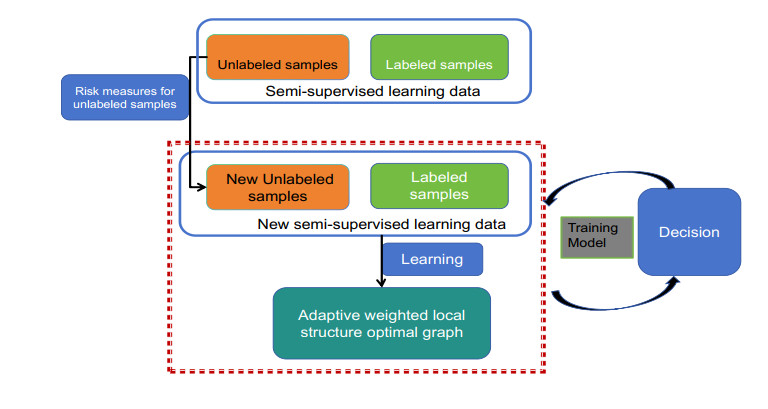
Manifold regularization semi-supervised learning is a powerful graph-based semi-supervised learning method. However, the performance of semi-supervised learning methods based on manifold regularization depends to some extent on the quality of the manifold graph and unlabeled samples. Intuitively speaking, the quality of the graph directly affects the final classification performance of the model. In response to the above problems, this paper first proposed an adaptive safety semi-supervised learning framework. The framework implements the weight assignment of the self-similarity graph during the model learning process. In order to adapt to the learning needs, accelerate the learning speed, and avoid the impact of the curse of dimensionality, the framework also optimizes the features of each sample point through an automatic weighting mechanism to extract effective features and eliminate redundant information in the learning task. In addition, the framework defines an adaptive risk measurement mechanism for the uncertainty and potential risks of unlabeled samples to determine the degree of risk of unlabeled samples. Finally, a new adaptive safe semi-supervised extreme learning machine was proposed. Comprehensive experimental results across various class imbalance scenarios demonstrated that our proposed method outperforms other methods in terms of classification accuracy, and other critical performance metrics.

| [1] | M. Belkin, P. Niyogi, V. Sindhwani, Manifold regularization: A geometric framework for learning from labeled and unlabeled examples, J. Mach. Learn. Res., 7 (2006), 2399–2434. |
| [2] | O. Chapelle, B. Schlkopf, A. Zien, Semi-supervised learning, Handbook on Neural Information Processing, Springer Berlin Heidelberg, 2013. |
| [3] |
Y. Wang, Y. Meng, Y. Li, S. Chen, Z. Fu, H. Xue, Semi-supervised manifold regularization with adaptive graph construction, Pattern Recog. Lett., 98 (2017), 90–95. https://doi.org/10.1016/j.patrec.2017.09.004 doi: 10.1016/j.patrec.2017.09.004

|
| [4] |
Z. Kang, H. Pan, S. C. Hoi, Z. Xu, Robust graph learning from noisy data, IEEE T. Cybernetics, 50 (2019), 1833–1843. https://doi.org/10.1109/TCYB.2018.2887094 doi: 10.1109/TCYB.2018.2887094
|
| [5] |
Z. Kang, C. Peng, Q. Cheng, X. Liu, X. Peng, Z. Xu, et al., Structured graph learning for clustering and semi-supervised classification, Pattern Recog., 110 (2021), 107627. https://doi.org/10.1016/j.patcog.2020.107627 doi: 10.1016/j.patcog.2020.107627
|
| [6] |
Z. Kang, X. Lu, Y. Lu, C. Peng, W. Chen, Z. Xu, Structure learning with similarity preserving, Neural Networks, 129 (2020), 138–148. https://doi.org/10.1016/j.neunet.2020.05.030 doi: 10.1016/j.neunet.2020.05.030
|
| [7] |
T. Yang, C. E. Priebe, The effect of model misspecification on semi-supervised classification, IEEE T. Pattern Anal., 33 (2011), 2093–2103. https://doi.org/10.1109/TPAMI.2011.45 doi: 10.1109/TPAMI.2011.45
|
| [8] |
Y. F. Li, Z. H. Zhou, Towards making unlabeled data never hurt, IEEE T. Pattern Anal., 37 (2015), 175–188. https://doi.org/10.1109/TPAMI.2014.2299812 doi: 10.1109/TPAMI.2014.2299812
|
| [9] | Y. F. Li, Z. H. Zhou, Improving semi-supervised support vector machines through unlabeled instances selection, In: Proceedings of the AAAI Conference on Artificial Intelligence, 25 (2011), 386–391. https://doi.org/10.1609/aaai.v25i1.7920 |
| [10] |
Y. Wang, S. Chen, Z. H. Zhou, New semi-supervised classification method based on modified cluster assumption, IEEE T. Neur. Net. Lear., 23 (2012), 689–702. https://doi.org/10.1109/TNNLS.2012.2186825 doi: 10.1109/TNNLS.2012.2186825
|
| [11] |
Y. Wang, S. Chen, Safety-aware semi-supervised classification, IEEE T. Neur. Net. Lear., 24 (2013), 1763–1772. https://doi.org/10.1109/TNNLS.2013.2263512 doi: 10.1109/TNNLS.2013.2263512
|
| [12] |
M. Kawakita, J. Takeuchi, Safe semi-supervised learning based on weighted likelihood, Neural Networks, 53 (2014), 146–164. https://doi.org/10.1016/j.neunet.2014.01.016 doi: 10.1016/j.neunet.2014.01.016
|
| [13] |
H. T. Gan, Z. Z. Luo, M. Meng, Y. Ma, Q. She, A risk degree-based safe semi-supervised learning algorithm, Int. J. Mach. Learn. Cyb., 7 (2015), 1–10. https://doi.org/10.1007/s13042-015-0416-8 doi: 10.1007/s13042-015-0416-8
|
| [14] |
H. T. Gan, Z. Luo, Y. Sun, X. Xi, N. Sang, R. Huang, Towards designing risk-based safe Laplacian regularized least squares, Expert Syst. Appl., 45 (2016), 1–7. https://doi.org/10.1016/j.eswa.2015.09.017 doi: 10.1016/j.eswa.2015.09.017
|
| [15] |
H. T. Gan, Z. Li, Y. Fan, Z. Luo, Dual learning-based safe semi-supervised learning, IEEE Access, 6 (2017), 2615–2621. https://doi.org/10.1109/ACCESS.2017.2784406 doi: 10.1109/ACCESS.2017.2784406
|
| [16] |
H. T. Gan, Z. Li, W. Wu, Z. Luo, R. Huang, Safety-aware graph-based semi-supervised learning, Expert Syst. Appl., 107 (2018), 243–254. https://doi.org/10.1016/j.eswa.2018.04.031 doi: 10.1016/j.eswa.2018.04.031
|
| [17] |
N. Sang, H. T. Gan, Y. Fan, W. Wu, Z. Yang, Adaptive safety degree-based safe semi-supervised learning, Int. J. Mach. Learn. Cyb., 10 (2018), 1101–1108. https://doi.org/10.1007/s13042-018-0788-7 doi: 10.1007/s13042-018-0788-7
|
| [18] |
Y. Wang, Y. Meng, Z. Fu, H. Xue, Towards safe semi-supervised classification: Adjusted cluster assumption via clustering, Neural Process. Lett., 46 (2017), 1031–1042. https://doi.org/10.1007/s11063-017-9607-5 doi: 10.1007/s11063-017-9607-5
|
| [19] |
H. T. Gan, G. Li, S. Xia, T. Wang, A hybrid safe semi-supervised learning method, Expert Syst. Appl., 149 (2020), 1–9. https://doi.org/10.1016/j.eswa.2020.113295 doi: 10.1016/j.eswa.2020.113295
|
| [20] | Y. T. Li, J. T. Kwok, Z. H. Zhou, Towards safe semi-supervised learning for multivariate performance measures, In: Proceedings of the Thirtieth AAAI Conference on Artificial Intelligence (AAAI'16), AAAI Press, 30 (2016), 1816–1822. https://doi.org/10.1609/aaai.v30i1.10282 |
| [21] |
G. Huang, S. Song, J. N. D. Gupta, C. Wu, Semi-supervised and unsupervised extreme learning machines, IEEE T. Cybernetics, 44 (2017), 2405–2417. https://doi.org/10.1109/TCYB.2014.2307349 doi: 10.1109/TCYB.2014.2307349
|
| [22] |
Q. She, B. Hu, H. Gan, Y. Fan, T. Nguyen, T. Potter, et al., Safe semi-supervised extreme learning machine for EEG signal classification, IEEE Access, 6 (2018), 49399–49407. https://doi.org/10.1109/ACCESS.2018.2868713 doi: 10.1109/ACCESS.2018.2868713
|
| [23] |
H. Xu, X. Wang, J. Huang, F. Zhang, F. Chu, Semi-supervised multi-sensor information fusion tailored graph embedded low-rank tensor learning machine under extremely low labeled rate, Inform. Fusion, 105 (2024), 102222. https://doi.org/10.1016/j.inffus.2023.102222 doi: 10.1016/j.inffus.2023.102222
|
| [24] |
J. Huang, F. Zhang, B. Safaei, Z. Qin, F. Chu, The flexible tensor singular value decomposition and its applications in multisensor signal fusion processing, Mech. Syst. Signal Pr., 220 (2024), 111662. https://doi.org/10.1016/j.ymssp.2024.111662 doi: 10.1016/j.ymssp.2024.111662
|
| [25] |
G. B. Huang, Q. Y. Zhu, C. K. Siew, Extreme learning machine: Theory and applications, Neurocomputing, 70 (2006), 489–501. https://doi.org/10.1016/j.neucom.2005.12.126 doi: 10.1016/j.neucom.2005.12.126
|
| [26] |
G. B. Huang, X. J. Ding, H. M. Zhou, Optimization method based extreme learning machine for classification, Neurocomputing, 74 (2010), 155–163. https://doi.org/10.1016/j.neucom.2010.02.019 doi: 10.1016/j.neucom.2010.02.019
|
| [27] |
Z. Liu, Z. Lai, W. Ou, K. Zhang, R. Zheng, Structured optimal graph based sparse feature extraction for semi-supervised learning, Signal Process., 170 (2020), 107456. https://doi.org/10.1016/j.sigpro.2020.107456 doi: 10.1016/j.sigpro.2020.107456
|
| [28] |
M. Luo, F. Nie, X. Chang, Y. Yang, A. G. Hauptmann, Q. Zheng, Adaptive unsupervised feature selection with structure regularization, IEEE T. Neur. Net. Lear., 29 (2018), 944–956. https://doi.org/10.1109/TNNLS.2017.2650978 doi: 10.1109/TNNLS.2017.2650978
|
| [29] |
J. S. Wu, M. X. Song, W. Min, J. H. Lai, W. S. Zheng, Joint adaptive manifold and embedding learning for unsupervised feature selection, Pattern Recog., 112 (2020), 107742. https://doi.org/10.1016/j.patcog.2020.107742 doi: 10.1016/j.patcog.2020.107742
|
| [30] |
F. Nie, W. Zhu, X. Li, Structured graph optimization for unsupervised feature selection, IEEE T. Knowl. Data En., 33 (2019), 1210–1222. https://doi.org/10.1109/TKDE.2019.2937924 doi: 10.1109/TKDE.2019.2937924
|
| [31] |
F. Nie, S. J. Shi, X. Li, Semi-supervised learning with auto-weighting feature and adaptive graph, IEEE T. Knowl. Data En., 32 (2019), 1167–1178. https://doi.org/10.1109/TKDE.2019.2901853 doi: 10.1109/TKDE.2019.2901853
|
| [32] | Q. Li, L. Jing, J. Yu, Adaptive graph constrained NMF for semi-supervised learning, In: Iapr International Workshop on Partially Supervised Learning, Springer, Berlin, Heidelberg, 2013, 36–48. https://doi.org/10.1007/978-3-642-40705-5_4 |
| [33] |
Y. Yuan, X. Li, Q. Wang, F. Nie, A semi-supervised learning algorithm via adaptive Laplacian graph, Neurocomputing, 426 (2020), 162–173. https://doi.org/10.1016/j.neucom.2020.09.069 doi: 10.1016/j.neucom.2020.09.069
|
| [34] |
Z. Liu, K. Shi, K. Zhang, W. Ou, L. Wang, Discriminative sparse embedding based on adaptive graph for dimension reduction, Eng. Appl. Artif. Intel., 94 (2020), 103758. https://doi.org/10.1016/j.engappai.2020.103758 doi: 10.1016/j.engappai.2020.103758
|


Figures(3) / Tables(7)

Jun Ma, Junjie Li, Jiachen Sun. A novel adaptive safe semi-supervised learning framework for pattern extraction and classification[J]. AIMS Mathematics, 2024, 9(11): 31444-31469. doi: 10.3934/math.20241514


 DownLoad: