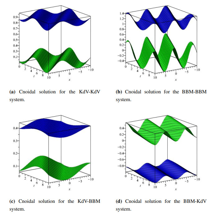
Some systems were recently put forth by Nguyen et al. as models for studying the interaction of long and short waves in dispersive media. These systems were shown to possess synchronized Jacobi elliptic solutions as well as synchronized solitary wave solutions under certain constraints, i.e., vector solutions, where the two components are proportional to one another. In this paper, the exact periodic traveling wave solutions to these systems in general were found to be given by Jacobi elliptic functions. Moreover, these cnoidal wave solutions are unique. Thus, the explicit synchronized solutions under some conditions obtained by Nguyen et al. are also indeed unique.
Citation: Bruce Brewer, Jake Daniels, Nghiem V. Nguyen. Exact Jacobi elliptic solutions of some models for the interaction of long and short waves[J]. AIMS Mathematics, 2024, 9(2): 2854-2873. doi: 10.3934/math.2024141
Some systems were recently put forth by Nguyen et al. as models for studying the interaction of long and short waves in dispersive media. These systems were shown to possess synchronized Jacobi elliptic solutions as well as synchronized solitary wave solutions under certain constraints, i.e., vector solutions, where the two components are proportional to one another. In this paper, the exact periodic traveling wave solutions to these systems in general were found to be given by Jacobi elliptic functions. Moreover, these cnoidal wave solutions are unique. Thus, the explicit synchronized solutions under some conditions obtained by Nguyen et al. are also indeed unique.

| [1] |
N. V. Nguyen, C. Y. Liu, Some models for the interaction of long and short waves in dispersive media. Part Ⅰ: Derivation, Water Waves, 2 (2020), 327–359. https://doi.org/10.1007/s42286-020-00038-6 doi: 10.1007/s42286-020-00038-6

|
| [2] |
C. Y. Liu, N. V. Nguyen, Some models for the interaction of long and short waves in dispersive media. Part Ⅱ: Well-posedness, Commun. Math. Sci., 21 (2023), 641–669. https://dx.doi.org/10.4310/CMS.2023.v21.n3.a3 doi: 10.4310/CMS.2023.v21.n3.a3
|
| [3] |
B. Deconinck, N. V. Nguyen, B. L. Segal, The interaction of long and short waves in dispersive media, J. Phys. A Math. Theor., 49 (2016), 415501. https://doi.org/10.1088/1751-8113/49/41/415501 doi: 10.1088/1751-8113/49/41/415501
|
| [4] |
T. Kawahara, N. Sugimoto, T. Kakutani, Nonlinear interaction between short and long capillary-gravity waves, J. Phys. Soc. Japan, 39 (1975), 1379–1386. https://doi.org/10.1143/JPSJ.39.1379 doi: 10.1143/JPSJ.39.1379
|
| [5] | C. Liu, N. V. Nguyen, B. Brewer, Explicit synchronized solitary waves for some models for the interaction of long and short waves in dispersive media, Adv. Differ. Equ., In press. |
| [6] | B. Brewer, C. Liu, N.V. Nguyen, Cnoidal wave solutions for some models for the interaction of long and short waves, In press. |
| [7] | M. A. Krasnosel'skii, Positive solutions of operator equations, Gronigan: P. Noordhoff Ltd., 1964. |
| [8] | M. A. Krasnosel'skii, Topological methods in the theory of nonlinear integral equations, London: Pergamon, 1964. |
| [9] |
H. Q. Chen, Existence of periodic traveling-wave solutions of nonlinear, dispersive wave equations, Nonlinearity, 17 (2004), 2041–2056. https://doi.org/10.1088/0951-7715/17/6/003 doi: 10.1088/0951-7715/17/6/003
|
| [10] |
H. Q. Chen, M. Chen, N. V. Nguyen, Cnoidal wave solutions to Boussinesq systems, Nonlinearity, 20 (2007), 1443–1461. https://doi.org/10.1088/0951-7715/20/6/007 doi: 10.1088/0951-7715/20/6/007
|
| [11] |
N. V. Nguyen, Existence of periodic traveling-wave solutions for a nonlinear Schrödinger system: a topological approach, Topol. Methods Nonlinear Anal., 43 (2016), 129–155. https://doi.org/10.12775/TMNA.2014.009 doi: 10.12775/TMNA.2014.009
|
| [12] |
M. Chen, Exact solutions of various Boussinesq systems, Appl. Math. Lett., 11 (1998), 45–49. https://doi.org/10.1016/S0893-9659(98)00078-0 doi: 10.1016/S0893-9659(98)00078-0
|
| [13] |
M. Chen, Exact traveling-wave solutions to bidirectional wave equations, Int. J. Theor. Phys., 37 (1998), 1547–1567. https://doi.org/10.1023/A:1026667903256 doi: 10.1023/A:1026667903256
|
| [14] |
J. L. Bona, M. Chen, J. C. Saut, Boussinesq equations and other systems for small-amplitude long waves in nonlinear dispersive media. Ⅰ: Derivation and linear theory, J. Nonlinear Sci., 12 (2002), 283–318. https://doi.org/10.1007/s00332-002-0466-4 doi: 10.1007/s00332-002-0466-4
|
| [15] |
J. L. Bona, M. Chen, J. C. Saut, Boussinesq equations and other systems for small-amplitude long waves in nonlinear dispersive media: Ⅱ. The nonlinear theory, Nonlinearity, 17 (2004), 925–952. https://doi.org/10.1088/0951-7715/17/3/010 doi: 10.1088/0951-7715/17/3/010
|
Figures(1)

Bruce Brewer, Jake Daniels, Nghiem V. Nguyen. Exact Jacobi elliptic solutions of some models for the interaction of long and short waves[J]. AIMS Mathematics, 2024, 9(2): 2854-2873. doi: 10.3934/math.2024141


 DownLoad: