Prescribed-time stabilization of nonlinear systems with uncertainties/disturbances by improved time-varying feedback control

Lichao Feng; Mengyuan Dai; Nan Ji; Yingli Zhang; Liping Du; Lichao Feng; Mengyuan Dai; Nan Ji; Yingli Zhang; Liping Du

doi:10.3934/math.20241159

AIMS Mathematics

2024, Volume 9, Issue 9: 23859-23877. doi: 10.3934/math.20241159

Previous Article Next Article

Research article Special Issues

Prescribed-time stabilization of nonlinear systems with uncertainties/disturbances by improved time-varying feedback control

1.
College of Science, North China University of Science and Technology, Tangshan 063210, China
2.
Hebei Key Laboratory of Data Science and Application, North China University of Science and Technology, Tangshan 063210, China

Received: 01 June 2024 Revised: 20 July 2024 Accepted: 07 August 2024 Published: 12 August 2024

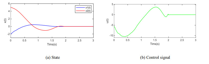
We address the prescribed-time stability of a class of nonlinear system with uncertainty/disturbance. With the help of the parametric Lyapunov equation (PLE), we designed a state feedback control to regulate the full-state of a controlled system within prescribed time, independent of initial conditions. The result illustrated that the controlled state converges to zero as $t$ approaches the settling time and remains zero thereafter. It was further proved that the controller is bounded by a constant that depends on the system state. A numerical example is presented to verify the validity of the theoretical results.
- nonlinear system,
- prescribed-time stability,
- state feedback,
- time-varying feedback control,
- parametric Lyapunov equation
Citation: Lichao Feng, Mengyuan Dai, Nan Ji, Yingli Zhang, Liping Du. Prescribed-time stabilization of nonlinear systems with uncertainties/disturbances by improved time-varying feedback control[J]. AIMS Mathematics, 2024, 9(9): 23859-23877. doi: 10.3934/math.20241159

Related Papers:

Abstract

We address the prescribed-time stability of a class of nonlinear system with uncertainty/disturbance. With the help of the parametric Lyapunov equation (PLE), we designed a state feedback control to regulate the full-state of a controlled system within prescribed time, independent of initial conditions. The result illustrated that the controlled state converges to zero as $t$ approaches the settling time and remains zero thereafter. It was further proved that the controller is bounded by a constant that depends on the system state. A numerical example is presented to verify the validity of the theoretical results.

References

[1]	M. B. Brilliant, Theory of the analysis of nonlinear systems, Technical report, Massachusetts Institute of Technology, Research Laboratory of Electronics, Cambridge, 1958.
[2]	S. Sastry, Nonlinear systems: analysis, stability, and control, New York: Springer, 1999. https://doi.org/10.1007/978-1-4757-3108-8
[3]	F. Amato, R. Ambrosino, M. Ariola, C. Cosentino, G. De Tommasi, Finite-time stability and control, London: Springer, 2014. https://doi.org/10.1007/978-1-4471-5664-2
[4]	X. Huang, W. Lin, B. Yang, Global finite-time stabilization of a class of uncertain nonlinear systems, Automatica, 41 (2005), 881–888. https://doi.org/10.1016/j.automatica.2004.11.036 doi: 10.1016/j.automatica.2004.11.036
[5]	Y Hong, Z. Jiang, Finite-time stabilization of nonlinear systems with parametric and dynamic uncertainties, IEEE Trans. Automat. Contr., 51 (2006), 1950–1956. https://doi.org/10.1109/TAC.2006.886515 doi: 10.1109/TAC.2006.886515
[6]	Y. Shen, Y. Huang, Global finite-time stabilization for a class of nonlinear systems, Int. J. Syst. Sci., 43 (2010), 73–78. https://doi.org/10.1080/00207721003770569 doi: 10.1080/00207721003770569
[7]	Z. Sun, L. Xue, K. Zhang, A new approach to finite-time adaptive stabilization of high-order uncertain nonlinear system, Automatica, 58 (2015), 60–66. https://doi.org/10.1016/j.automatica.2015.05.005 doi: 10.1016/j.automatica.2015.05.005
[8]	Y. Shtessel, C. Edwards, L. Fridman, A. Levant, Sliding mode control and observation, New York: Birkhäuser, 2014. https://doi.org/10.1007/978-0-8176-4893-0
[9]	S. Ding, A. Levant, S. Li, Simple homogeneous sliding-mode controller, Automatica, 67 (2016), 22–32. https://doi.org/10.1016/j.automatica.2016.01.017 doi: 10.1016/j.automatica.2016.01.017
[10]	S. P. Bhat, D. S. Bernstein, Finite-time stability of continuous autonomous systems, SIAM J. Control Optim., 38 (2000), 751–766. https://doi.org/10.1137/S0363012997321358 doi: 10.1137/S0363012997321358
[11]	Z. Y. Sun, Y. Shao, C. C. Chen, Fast finite-time stability and its application in adaptive control of high-order nonlinear system, Automatica, 106 (2019), 339–348. https://doi.org/10.1016/j.automatica.2019.05.018 doi: 10.1016/j.automatica.2019.05.018
[12]	Y. Hong, Finite-time stabilization and stabilizability of a class of controllable systems, Syst. Control Lett., 46 (2002), 231–236. https://doi.org/10.1016/S0167-6911(02)00119-6 doi: 10.1016/S0167-6911(02)00119-6
[13]	S. P. Bhat, D. S. Bernstein. Geometric homogeneity with applications to finite-time stability, Math. Control Signals Syst., 17 (2005), 101–127. https://doi.org/10.1007/s00498-005-0151-x doi: 10.1007/s00498-005-0151-x
[14]	A. Polyakov, D. Efimov, W. Perruquetti, Finite-time and fixed-time stabilization: implicit Lyapunov function approach, Automatica, 51 (2015), https://doi.org/10.1016/j.automatica.2014.10.082
[15]	W. Lin, C. C. Qian, Adding a power integrator: a tool for global stabilization of high-order lower-triangular systems, Syst. Control Lett., 39 (2000), 339–351. https://doi.org/10.1016/S0167-6911(99)00115-2 doi: 10.1016/S0167-6911(99)00115-2
[16]	C. Hu, J. Yu, Z. Chen, H. J. Jiang, T. W. Huang, Fixed-time stability of dynamical systems and fixed-time synchronization of coupled discontinuous neural networks, Neural Net., 89 (2017), 74–83. https://doi.org/10.1016/j.neunet.2017.02.001 doi: 10.1016/j.neunet.2017.02.001
[17]	A. Polyakov, Nonlinear feedback design for fixed-time stabilization of linear control systems, IEEE Trans. Automat. Contr., 57 (2011), 2106–2110. https://doi.org/10.1109/TAC.2011.2179869 doi: 10.1109/TAC.2011.2179869
[18]	K. Zimenko, A, Polyakov, D. Efimov, W. Perruquetti, On simple scheme of finite/fixed-time control design, Int. J. Control, 93 (2020), 1353–1361. https://doi.org/10.1080/00207179.2018.1506889 doi: 10.1080/00207179.2018.1506889
[19]	Z. Zuo, Q. L. Han, B. Ning, X. Ge, X. M, Zhang, An overview of recent advances in fixed-time cooperative control of multiagent systems, IEEE Trans. Ind. Inf., 14 (2018), 2322–2334. https://doi.org/10.1109/TⅡ.2018.2817248 doi: 10.1109/TⅡ.2018.2817248
[20]	C. C. Chen, Z. Y. Sun, Fixed-time stabilization for a class of high-order non-linear systems, IET Control Theory Appl., 12 (2018), 2578–2587. https://doi.org/10.1049/iet-cta.2018.5053 doi: 10.1049/iet-cta.2018.5053
[21]	B. Ning, Q. Han, Z. Zuo, L. Ding, Q. Lu, X. Ge, Fixed-time and prescribed-time consensus control of multiagent systems and its applications: a survey of recent trends and methodologies, IEEE Trans. Ind. Inf., 19 (2022), 1121–1135. https://doi.org/10.1109/TⅡ.2022.3201589 doi: 10.1109/TⅡ.2022.3201589
[22]	X. Li, C. Wen, J. Wang, Lyapunov-based fixed-time stabilization control of quantum systems, J. Autom. Intell., 1 (2022), 100005. https://doi.org/10.1016/j.jai.2022.100005 doi: 10.1016/j.jai.2022.100005
[23]	P. Zarchan, Tactical and strategic missile guidance, 6 Eds., American Institute of Aeronautics and Astronautics, Inc., 2012. https://doi.org/10.2514/4.868948
[24]	Y. D. Song, Y. Wang, J. Holloway, M. Krstic, Time-varying feedback for regulation of normal-form nonlinear systems in prescribed finite time, Automatica, 83 (2017), 243–251. https://doi.org/10.1016/j.automatica.2017.06.008 doi: 10.1016/j.automatica.2017.06.008
[25]	Y. D. Song, Y. Wang, M. Krstic, Time-varying feedback for stabilization in prescribed finite time, Int. J. Robust Nonlinear Contr., 29 (2019), 618–633. https://doi.org/10.1002/rnc.4084 doi: 10.1002/rnc.4084
[26]	D. Tran, T. Yucelen, S. B. Sarsilmaz, Finite-time control of multiagent networks as systems with time transformation and separation principle, Control Eng. Pract., 108 (2021), 104717. https://doi.org/10.1016/j.conengprac.2020.104717 doi: 10.1016/j.conengprac.2020.104717
[27]	K. Zhao, Y. Song, Y. Wang, Regular error feedback based adaptive practical prescribed time tracking control of normal-form nonaffine systems, J. Franklin Inst., 356 (2019), 2759–2779. https://doi.org/10.1016/j.jfranklin.2019.02.015 doi: 10.1016/j.jfranklin.2019.02.015
[28]	Y. Wang, Y. D. Song. A general approach to precise tracking of nonlinear systems subject to non-vanishing uncertainties, Automatica, 106 (2019), 306–314. https://doi.org/10.1016/j.automatica.2019.05.008 doi: 10.1016/j.automatica.2019.05.008
[29]	W. Li, M. Krstic, Stochastic nonlinear prescribed-time stabilization and inverse optimality, IEEE Trans. Automat. Contr., 67 (2021), 1179–1193. https://doi.org/10.1109/TAC.2021.3061646 doi: 10.1109/TAC.2021.3061646
[30]	H. Ye, Y. Song, Prescribed-time control for linear systems in canonical form via nonlinear feedback, IEEE Trans. Syst. Man Cyber.: Syst., 53 (2023), 1126–1135. https://doi.org/10.1109/TSMC.2022.3194908 doi: 10.1109/TSMC.2022.3194908
[31]	F. Gao, Y. Wu, Z. Zhang, Global fixed-time stabilization of switched nonlinear systems: a time-varying scaling transformation approach, IEEE Trans. Circuits Syst. Ⅱ: Express Briefs, 66 (2019), 1890–1894. https://doi.org/10.1109/TCSⅡ.2018.2890556 doi: 10.1109/TCSⅡ.2018.2890556
[32]	J. Tsinias, A theorem on global stabilization of nonlinear systems by linear feedback, Syst. Control Lett., 17 (1991), 357–362. https://doi.org/10.1016/0167-6911(91)90135-2 doi: 10.1016/0167-6911(91)90135-2
[33]	J. Holloway, M. Krstic, Prescribed-time observers for linear systems in observer canonical form, IEEE Trans. Automat. Contr., 64 (2019), 3905–3912. https://doi.org/10.1109/TAC.2018.2890751 doi: 10.1109/TAC.2018.2890751
[34]	P. Krishnamurthy, F. Khorrami, M. Krstic, A dynamic high-gain design for prescribed-time regulation of nonlinear systems, Automatica, 115 (2020), 108860. https://doi.org/10.1016/j.automatica.2020.108860 doi: 10.1016/j.automatica.2020.108860
[35]	E. Jiménez-Rodríguez, A. J. Muñoz-Vázquez, J. D. Sánchez-Torres, M. Defoort, A. G. Loukianov, A Lyapunov-like characterization of predefined-time stability, IEEE Trans. Automat. Contr., 65 (2020), 4922–4927. https://doi.org/10.1109/TAC.2020.2967555 doi: 10.1109/TAC.2020.2967555
[36]	B. Zhou, Finite-time stabilization of linear systems by bounded linear time-varying feedback, Automatica, 113 (2020), 108760. https://doi.org/10.1016/j.automatica.2019.108760 doi: 10.1016/j.automatica.2019.108760
[37]	B. Zhou, Y. Shi, Prescribed-time stabilization of a class of nonlinear systems by linear time-varying feedback, IEEE Trans. Automat. Contr., 66 (2021), 6123–6130. https://doi.org/10.1109/TAC.2021.3061645 doi: 10.1109/TAC.2021.3061645
[38]	K. K. Zhang, B. Zhou, G, Duan, Prescribed-time input-to-state stabilization of normal nonlinear systems by bounded time-varying feedback, IEEE Trans. Circuits Syst. I, 69 (2022), 3715–3725. https://doi.org/10.1109/TCSI.2022.3182884 doi: 10.1109/TCSI.2022.3182884
[39]	C. C. Chen, C. J. Qian, Z. Y. Sun, Y. W. Yang, Global output feedback stabilization of a class of nonlinear systems with unknown measurement sensitivity, IEEE Trans. Automat. Contr., 63 (2017), 2212–2217. https://doi.org/10.1109/TAC.2017.2759274 doi: 10.1109/TAC.2017.2759274
[40]	Z. Sheng, Q. Ma, S. Xu, Prescribed-time output feedback control for high-order nonlinear systems, IEEE Trans. Circuits Syst. Ⅱ: Express Briefs, 70 (2023), 2460–2464. https://doi.org/10.1109/TCSⅡ.2023.3241160 doi: 10.1109/TCSⅡ.2023.3241160
[41]	X. He, X. Li, S. Song, Prescribed-time stabilization of nonlinear systems via impulsive regulation, IEEE Trans. Syst. Man Cyber.: Syst., 53 (2022), 981–985. https://doi.org/10.1109/TSMC.2022.3188874 doi: 10.1109/TSMC.2022.3188874
[42]	B. Zhou, K. K. Zhang, A linear time-varying inequality approach for prescribed time stability and stabilization, IEEE Trans. Cyber., 53 (2022), 1880–1889. https://doi.org/10.1109/TCYB.2022.3164658 doi: 10.1109/TCYB.2022.3164658

Reader Comments

Your name:*

Email:*
© 2024 the Author(s), licensee AIMS Press. This is an open access article distributed under the terms of the Creative Commons Attribution License (http://creativecommons.org/licenses/by/4.0)