Chaos and stability of a fractional model of the cyber ecosystem

José F. Gómez-Aguilar; Manisha Krishna Naik; Reny George; Chandrali Baishya; İbrahim Avcı; Eduardo Pérez-Careta; José F. Gómez-Aguilar; Manisha Krishna Naik; Reny George; Chandrali Baishya; İbrahim Avcı; Eduardo Pérez-Careta

doi:10.3934/math.20241077

AIMS Mathematics

2024, Volume 9, Issue 8: 22146-22173. doi: 10.3934/math.20241077

Previous Article Next Article

Research article Special Issues

Chaos and stability of a fractional model of the cyber ecosystem

1.
Centro de Investigación en Ingeniería y Ciencias Aplicadas (CIICAp-IICBA), Universidad Autónoma del Estado de Morelos, Av. Universidad 1001, Col. Chamilpa, C.P. 62209 Cuernavaca, Morelos, México
2.
Department of Studies and Research in Mathematics, Tumkur University, Tumkur-572103, Karnataka, India
3.
Department of Mathematics, College of Science and Humanities in Al-Kharj, Prince Sattam bin Abdulaziz University, Al-Kharj 11942, Saudi Arabia
4.
Department of Computer Engineering, Faculty of Engineering, Final International University, Kyrenia, Northern Cyprus, via Mersin 10, Turkey
5.
Universidad de Guanajuato, Dpto. Electrónica, Carretera Salamanca-Valle de Santiago, Km 3+1.8, Salamanca Gto, México

Received: 29 April 2024 Revised: 17 June 2024 Accepted: 01 July 2024 Published: 16 July 2024
MSC : 65P20, 92D40, 26A33, 34D08

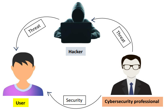
The widespread use of computer hardware and software in society has led to the emergence of a type of criminal conduct known as cybercrime, which has become a major worldwide concern in the 21st century spanning multiple domains. As a result, in the present setting, academics and practitioners are showing a great deal of interest in conducting research on cybercrime. In this work, a fractional-order model was replaced by involving three sorts of human populations: online computer users, hackers, and cyber security professionals, in order to examine the online computer user-hacker system. The existence, uniqueness and boundedness were studied. To support our theoretical conclusions, a numerical analysis of the influence of the various logical parameters was conducted and we derived the necessary conditions for the different equilibrium points to be locally stable. We examined the effects of the fear level and refuge factor on the equilibrium densities of prey and predators in order to explore and understand the dynamics of the system in a better way. Using some special circumstances, the model was examined. Our theoretical findings and logical parameters were validated through a numerical analysis utilizing the generalized Adams-Bashforth-Moulton technique.

Keywords:

Citation: José F. Gómez-Aguilar, Manisha Krishna Naik, Reny George, Chandrali Baishya, İbrahim Avcı, Eduardo Pérez-Careta. Chaos and stability of a fractional model of the cyber ecosystem[J]. AIMS Mathematics, 2024, 9(8): 22146-22173. doi: 10.3934/math.20241077

Related Papers:

[1]	Cuiying Li, Rui Wu, Ranzhuo Ma . Existence of solutions for Caputo fractional iterative equations under several boundary value conditions. AIMS Mathematics, 2023, 8(1): 317-339. doi: 10.3934/math.2023015
[2]	Ahmed Alsaedi, Fawziah M. Alotaibi, Bashir Ahmad . Analysis of nonlinear coupled Caputo fractional differential equations with boundary conditions in terms of sum and difference of the governing functions. AIMS Mathematics, 2022, 7(5): 8314-8329. doi: 10.3934/math.2022463
[3]	Murat A. Sultanov, Vladimir E. Misilov, Makhmud A. Sadybekov . Numerical method for solving the subdiffusion differential equation with nonlocal boundary conditions. AIMS Mathematics, 2024, 9(12): 36385-36404. doi: 10.3934/math.20241726
[4]	Naimi Abdellouahab, Keltum Bouhali, Loay Alkhalifa, Khaled Zennir . Existence and stability analysis of a problem of the Caputo fractional derivative with mixed conditions. AIMS Mathematics, 2025, 10(3): 6805-6826. doi: 10.3934/math.2025312
[5]	Xinwei Su, Shuqin Zhang, Lixin Zhang . Periodic boundary value problem involving sequential fractional derivatives in Banach space. AIMS Mathematics, 2020, 5(6): 7510-7530. doi: 10.3934/math.2020481
[6]	Ayub Samadi, Chaiyod Kamthorncharoen, Sotiris K. Ntouyas, Jessada Tariboon . Mixed Erdélyi-Kober and Caputo fractional differential equations with nonlocal non-separated boundary conditions. AIMS Mathematics, 2024, 9(11): 32904-32920. doi: 10.3934/math.20241574
[7]	Karim Guida, Lahcen Ibnelazyz, Khalid Hilal, Said Melliani . Existence and uniqueness results for sequential $\psi$ -Hilfer fractional pantograph differential equations with mixed nonlocal boundary conditions. AIMS Mathematics, 2021, 6(8): 8239-8255. doi: 10.3934/math.2021477
[8]	Nichaphat Patanarapeelert, Thanin Sitthiwiratthame . On nonlocal fractional symmetric Hanh integral boundary value problems for fractional symmetric Hahn integrodifference equation. AIMS Mathematics, 2020, 5(4): 3556-3572. doi: 10.3934/math.2020231
[9]	Abdelkader Amara . Existence results for hybrid fractional differential equations with three-point boundary conditions. AIMS Mathematics, 2020, 5(2): 1074-1088. doi: 10.3934/math.2020075
[10]	Yige Zhao, Yibing Sun, Zhi Liu, Yilin Wang . Solvability for boundary value problems of nonlinear fractional differential equations with mixed perturbations of the second type. AIMS Mathematics, 2020, 5(1): 557-567. doi: 10.3934/math.2020037

Abstract

1. Introduction

In graph theory, graph labeling is an assignment of labels or weights to the vertices and edges of a graph. Graph labeling plays an important role in many fields such as computer science, coding theory and physics ^[32]. Baca et al. ^[10] have introduced the definition of an edge irregular total $\ell$ -labeling of any graph as a labeling $\mathcal{L}:V \cup E\to \left\{\mathrm{1, 2}, 3, \dots, \ell\right\}$ in which every two distinct edges $fh$ and ${f}^{*}{h}^{*}$ of a graph $G$ have distinct weights, this means that ${w}_{\mathcal{L}}\left(fh\right)\ne {w}_{\mathcal{L}}\left({f}^{*}{h}^{*}\right)$ where ${w}_{\mathcal{L}}\left(fh\right) = \mathcal{L}\left(f\right)+\mathcal{L}\left(h\right)+\mathcal{L}\left(fh\right)$ . They have deduced inequality which gives a lower bound of $tes\left(G\right)$ for a graph $G$ ,

$tes\left(G\right)\ge max\left\{\left\lceil {\frac{\left|E\left(G\right)\right|+2}{3}} \right\rceil , \left\lceil {\frac{\Delta +1}{2}} \right\rceil \right\}$

(1)

Also, they have introduced the exact value of TEIS, $tes\left(G\right)$ for some families of graphs like fan graph ${F}_{n}$ and wheel graph ${W}_{n}$ ,

$tes\left({F}_{n}\right) = \left\lceil {\frac{3n+2}{3}} \right\rceil \text{, }$

$tes\left({W}_{n}\right) = \left\lceil {\frac{2n+2}{3}} \right\rceil \text{.}$

In ^[15] authors have proved that for any tree $T$

$tes\left(T\right) = max\left\{\left\lceil {\frac{k+1}{3}} \right\rceil , \left\lceil {\frac{\Delta +1}{2}} \right\rceil \right\},$

where $\Delta$ is maximum degree on $k$ vertices. In addition, Salama ^[26] investigated the exact value of TEIS for a polar grid graph,

$tes\left({P}_{m, n}\right) = \left\lceil {\frac{2mn+2}{3}} \right\rceil \text{.}$

Authors in ^[1] determined $\mathrm{T}\mathrm{E}\mathrm{I}\mathrm{S}$ for zigzag graphs. Also, the exact value of TEIS of the generalized web graph ${W}_{n, m}$ and some families has been determined, see ^[14]. Tilukay et al. ^[31] have investigated total irregularity strength for a wheel graph, a fan graph, a triangular Book graph and a friendship graph. On the other hand, in ^{[2,3,8,17,20,24,29]} the total edge irregularity strengths for hexagonal grid graphs, centralized uniform theta graphs, generalized helm graph, series parallel graphs, disjoint union of isomorphic copies of generalized Petersen graph, disjoint union of wheel graphs, subdivision of star ${S}_{n}$ and categorical product of two cycles have been investigated. For more details, see ^{[4,5,6,7,9,11,12,13,16,18,19,21,23,25,27,28,30]}.

A generalized theta graph $\theta ({t}_{1}, {t}_{2}, \dots, {t}_{n})$ is a pair of $n$ internal disjoint paths with lengths at least two joined by end vertices where the end vertices are named south pole $S$ and north pole $N$ and ${t}_{i}$ is the number of vertices in the nth path. Uniform theta graph $\theta (t, m)$ is a generalized theta graph in which all paths have the same numbers of internal vertices, for more details see ^[22].

In this paper, we have defined a new type of family of graph called uniform theta snake graph, ${\theta }_{n}(t, m)$ . Also, the exact value of TEIS for some special types of the new family has been determined.

2. Main results

In the following, we define a new type of graph which is called uniform theta snake graph.

Definition 1. If we replace each edge of a path ${P}_{n}$ by a uniform theta graph $\theta (t, m)$ , we have a uniform theta snake graph ${\theta }_{n}(t, m)$ . See Figure 1.

Figure 1. Uniform theta snake graph θ(t, m).

DownLoad: Full-Size Img PowerPoint

It is clear that for a uniform theta snake graph $\left|\mathrm{E}\left({\mathtt{θ }}_{\mathrm{n}}\right(\mathrm{t}, \mathrm{m}\left)\right)\right| = \mathrm{t}\left(\mathrm{m}+1\right)\mathrm{n}$ and $\left|\mathrm{V}\left({\mathtt{θ }}_{\mathrm{n}}\right(\mathrm{t}, \mathrm{m}\left)\right)\right| = \left(\mathrm{t}\mathrm{m}+1\right)\mathrm{n}+1$ . In this section, we determine the exact value of TEIS for uniform theta snake graph ${\mathtt{θ }}_{\mathrm{n}}\left(\mathrm{3, 3}\right)$ , ${\mathtt{θ }}_{\mathrm{n}}\left(3, \mathrm{m}\right)$ , ${\mathtt{θ }}_{\mathrm{n}}(\mathrm{t}, 3)$ , ${\mathtt{θ }}_{\mathrm{n}}\left(4, \mathrm{m}\right)$ , and ${\mathtt{θ }}_{\mathrm{n}}(\mathrm{t}, 4)$ .

Theorem 1. For a uniform theta snake graph ${\theta }_{n}\left(\mathrm{3, 3}\right)$ with 10 $n+1$ vertices and 12 $n$ edges, we have

$tes\left({\theta }_{n}\left(\mathrm{3, 3}\right)\right) = 4n+1\text{.}$

Proof. Since a uniform theta snake graph ${\theta }_{n}\left(\mathrm{3, 3}\right)$ has 12 $n$ edges and $\left({\theta }_{n}\left(\mathrm{3, 3}\right)\right) = 6$ , then from (1) we have:

$tes\left({\theta }_{n}\left(\mathrm{3, 3}\right)\right)\ge 4n+1\text{.}$

To prove the invers inequality, we show that $ħ-$ labeling is an edge irregular total for ${\theta }_{n}\left(\mathrm{3, 3}\right)$ , see , and $ħ = 4n+1$ . Let $ħ = 4n+1$ and a total $ħ-$ labeling $\alpha :V{(\theta }_{n}\left(\mathrm{3, 3}\right)) \cup E({\theta }_{n}\left(\mathrm{3, 3}\right))\to \left\{\mathrm{1, 2}, 3, \dots, \mathrm{ħ}\right\}$ is defined as:

Figure 2. Uniform theta snake graph θ(3, 3).

DownLoad: Full-Size Img PowerPoint

$\mathtt{α }\left({\mathrm{c}}_{0}\right) = 1,$

$\mathtt{α }\left({\mathrm{c}}_{\mathrm{s}}\right) = 4\mathrm{s}\mathrm{ }\mathrm{ }\mathrm{ }\mathrm{ }\mathrm{ }\mathrm{ }\mathrm{ }\mathrm{ }\mathrm{ }\mathrm{ }\mathrm{ }\mathrm{ }\;\mathrm{f}\mathrm{o}\mathrm{r}\;\mathrm{ }1\le \mathrm{s}\le \mathrm{n}-1$

$\mathtt{α }\left({\mathrm{c}}_{\mathrm{n}}\right) = \mathrm{ħ},$

$\alpha \left({x}_{i, j}\right) = \left\{\begin{array}{cc}j& for\;1\le j\le 3\\ j+1& for\;4\le j\le 6\\ .& .\\ .& .\\ j+n-1& for\;3n-2\le j\le 3n-1\end{array}, i = 1, \mathrm{ }2, \mathrm{ }3\right.\text{, }$

$\alpha \left({x}_{i, 3n}\right) = ħ-1 \; for\; i = 1, 2, 3$

$\alpha \left({c}_{0}{x}_{i, 1}\right) = i \; for\; i = i1, 2, 3$

$\alpha \left({c}_{S}{x}_{i, 3S}\right) = 4S+i \; for\; 1\le S\le n-1, i = 1, 2, 3$

$\alpha \left({c}_{S}{x}_{i, 3S+1}\right) = 4S+i+1 \; for\; 1\le S\le n-1, i = 1, 2, 3$

$\alpha \left({c}_{n}{x}_{i, 3n}\right) = \left\{\begin{array}{cc}ħ-2& for\; i = 1\\ ħ-1& for\; i = 2\\ ħ& for\; i = 3\end{array}\right.\text{, }$

$\alpha \left({{x}_{i, j}x}_{i, j+1i}\right) = \left\{\begin{array}{cc}j+i+1& for\; 1\le j\le 2\\ j+i+2& for\; 4\le j\le 5\\ .& .\\ .& .\\ j+i+n-\mathrm{I}1& for\; 3n-5\le j\le 3n-4\\ ħ+i-3& for\; 3n-2\le j\le 3n-1\end{array}, i = 1, 2, 3\right..$

It is clear that $ħ$ is the greatest used label. The weights of edges of ${\theta }_{n}\left(\mathrm{3, 3}\right)$ are given by:

${w}_{\alpha }\left({c}_{0}{x}_{i, 1}\right) = i+2 \; for\; i = 1, 2, 3\text{, }$

${w}_{\alpha }\left({c}_{S}{x}_{i, 3S}\right) = 12S+i-1 \; for\; 1\le S\le n-1 , i = 1, 2, 3$

${w}_{\alpha }\left({c}_{S}{x}_{i, 3S+1}\right) = 12S+i+2\; for\; 1\le S\le n-1, i = 1, 2, 3,$

${w}_{\alpha }\left({c}_{n}{x}_{i, 3n}\right) = \left\{\begin{array}{cc}3\left(ħ-1\right)& for\; i = 1\\ 3ħ-2& for\; i = 2\\ 3ħ-1& for\; i = 3\end{array}\right.\text{, }$

${w}_{\alpha }\left({{x}_{i, j}x}_{i, j+1}\right) = \left\{\begin{array}{cc}3j+i+2& for\; 1\le j\le 2\\ 3j+i+5& for\; 4\le j\le 5\\ .& .\\ .& .\\ 3j+i+3n-4& for\; 3n-5\le j\le 3n-4\\ 3ħ+i-10& for\; j = 3n-2\\ 3ħ+i-7& for\; j = 3n-1\end{array}, i = 1, 2, 3\right.$

Obviously, the weights of edges are distinct. So $\alpha$ is an edge irregular total $\mathrm{ħ}-$ labeling. Hence

$tes\left({\theta }_{n}\left(\mathrm{3, 3}\right)\right) = 4n+1\text{.}$

Theorem 2. For ${\theta }_{n}\left(3, m\right), m>3$ be a uniform theta snake graph. Then

$tes\left({\theta }_{n}(3, m)\right) = (m+1)n+1\text{.}$

Proof. Since $\left|E\left({\theta }_{n}\right(3, m\left)\right)\right| = 3\left(m+1\right)n$ and $\Delta \left({\theta }_{n}\right(3, m\left)\right) = 6$ . Substituting in (1), we find

$tes\left({\theta }_{n}(3, m)\right)\ge (m+1)n+1\text{.}$

The existence of an edge irregular total $ƛ-$ labeling for ${\theta }_{n}(3, m)$ , See , $m>3$ will be shown, with $ƛ = (m+1)n+1$ . Define a total $ƛ-$ labeling $\beta :V\left({\theta }_{n}(3, m)\right)\cup E\left({\theta }_{n}(3, m)\right)\to \left\{\mathrm{1, 2}, 3, \dots, ƛ\right\}$ for ${\theta }_{n}(3, m)$ as:

Figure 3. Uniform theta snake graph θ(3, m).

DownLoad: Full-Size Img PowerPoint

$\beta \left({c}_{0}\right) = 1,$

$\beta \left({c}_{s}\right) = (m+1)s \; for\; 1\le s\le n-1\text{, }$

$\beta \left({c}_{n}\right) = ƛ$

$\beta \left({x}_{i, j}\right) = \left\{\begin{array}{cc}j& for\; 1\le j\le m\\ j+1& for\; m+1\le j\le 2m\\ .& .\\ .& .\\ j+n-1& for\; m\left(n-1\right)+1\le j\le mn-1\end{array}\right.\text{, }$

$\beta \left({x}_{i, mn}\right) = ƛ-1 \; for\; i = 1, 2, 3$

$\beta \left({c}_{0}{x}_{i, 1}\right) = 1 \; for\; i = 1, 2, 3$

$\beta \left({c}_{S}{x}_{i, mS}\right) = (m+1)S+i \; for\; 1\le S\le n-1, i = 1, 2, 3$

$\beta \left({c}_{S}{x}_{i, mS+1}\right) = (m+1)S+i+1 \; for\; 1\le S\le n-1, i = 1, 2, 3$

$\beta \left({c}_{n}{x}_{i, mn}\right) = \left\{\begin{array}{cc}ƛ-2& for\; i = 1\\ ƛ-1& for\; i = 2\\ ƛ& for\; i = 3\end{array}\right.\text{, }$

$\beta \left({{x}_{i, j}x}_{i, j+1}\right) = \left\{\begin{array}{cc}j+i+1& for\; 1\le j\le m-1\\ j+i+2& for\; m+1\le j\le 2m-1\\ .& .\\ .& .\\ j+i+n& for\; m\left(n-1\right)+1\le j\le mn-2\\ j+i+n-1& for\; j = mn-1\end{array}.\right.$

Clearly, $ƛ$ is the most label of edges and vertices. The edges weights are given as follows:

${w}_{\beta }\left({c}_{0}{x}_{i, 1}\right) = i+2\; for\; i = 1, 2, 3\text{, }$

${w}_{\beta }\left({c}_{S}{x}_{i, mS}\right) = 3\left(m+1\right)S+i-1 \; for\; 1\le S\le n-1, i = 1, 2, 3$

${w}_{\beta }\left({c}_{S}{x}_{i, mS+1}\right) = 3\left(m+1\right)S+i+2 \; for\; 1\le S\le n-1, i = 1, 2, 3\text{, }$

${w}_{\beta }\left({c}_{n}{x}_{i, mn}\right) = \left\{\begin{array}{cc}3ƛ-3& for\; i = 1\\ 3ƛ-2& for\; i = 2\\ 3ƛ-1& for\; i = 3\end{array}\right.\text{, }$

${w}_{\beta }\left({{x}_{i, j}x}_{i, j+1}\right) = \left\{\begin{array}{cc}3j+i+2& for\; 1\le j\le m-1\\ 3j+i+5& for\; m+1\le j\le 2m-1\\ .& .\\ .& .\\ 3j\mathrm{I}+i+3n-1& for\; m\left(n-1\right)+1\le j\le mn-2\\ 3ƛ+i-7& for\; j = mn-1\end{array}, \right.$

It is obvious that the weights of edges are different, thus $\beta$ is an edge irregular total $ƛ-$ labeling of ${\theta }_{n}(3, m)$ . Hence

$tes\left({\theta }_{n}(3, m)\right) = (m+1)n+1\text{.}$

Theorem 3. Let ${\theta }_{n}\left(t, 3\right)$ be a theta snake graph for $t>3$ . Then

$tes\left({\theta }_{n}(t, 3)\right) = \left\lceil {\frac{4tn+2}{3}} \right\rceil \text{.}$

Proof. A size of the graph ${\theta }_{n}(t, 3)$ equals $4tn$ and $\Delta \left({\theta }_{n}\left(t, 3\right)\right) = 2t$ , then from (1) we have

$tes\left({\theta }_{n}(t, 3)\right)\ge \left\lceil {\frac{4tn+2}{3}} \right\rceil \text{.}$

We define an edge irregular total $ħ-$ labeling for ${\theta }_{n}(t, 3)$ to get upper bound. So, let $ħ = \left\lceil {\frac{4tn+2}{3}} \right\rceil$ and a total $ħ-$ labeling $\gamma :V\left({\theta }_{n}(t, 3)\right)\cup E\left({\theta }_{n}(t, 3)\right)\to \left\{\mathrm{1, 2}, 3, \dots, ħ\right\}$ is defined in the following three cases:

Case 1. $4tn+2\equiv 0\left(mod \; 3\right)$

$\gamma$ is defined as:

$\gamma \left({c}_{0}\right) = 1,$

$\gamma \left({c}_{S}\right) = \left(t+1\right)S\; for\; 1\le S\le n-1\text{, }$

$\gamma \left({c}_{n}\right) = ħ$

$\gamma \left({x}_{i, j}\right)\mathrm{I} = \left\{\begin{array}{cc}i& for\; 1\le j\le 3, i = 1, 2, \dots , t\\ i+t+1& for\; 4\le j\le 6, i = 1, 2, \dots , t\\ i+2(t+1)& for\; 7\le j\le 9, i = 1, 2, \dots , t\\ .& .\\ .& .\\ .& .\\ i+(n-1)(t+1)& for\; 3n-5\le j\le 3n-3, i = 1, 2, \dots , t\\ ħ-1& for\; 3n-2\le j\le 3n, i = 1\\ ħ& for\; 3n-2\le j\le 3n, i = 2, 3, \dots , t\end{array}\right.\text{, }$

$\gamma \left({c}_{0}{x}_{i, 1}\right) = 1 \; for\; i = 1, 2, \dots , t$

$\gamma \left({c}_{S}{x}_{i, 3S}\right) = 2St-2S+3 \; for\; 1\le S\le n-1, i = 1, 2, \dots , t$

$\gamma \left({c}_{n}{x}_{i, 3n}\right) = \left\{\begin{array}{cc}ħ-t+2& for\; i = 1\\ ħ-t+i& for\; i = 2, 3, \dots , t\end{array}\right.\text{, }$

$\gamma \left({c}_{S}{x}_{i, 3S+1}\right) = 2St-2S+2 \; for\; 1\le S\le n-1, i = 1, 2, \dots , t$

$\gamma \left({{c}_{n-1}x}_{i, 3n-2}\right) = \left\{\begin{array}{c}\left\{\begin{array}{cc}\left(t+2\right)n-t-5& for\; i = 1\\ \left(t+2\right)n-t+i-7& for\; i = 2, 3, \dots , t\end{array}, n = 2, 3\right.\\ \begin{array}{c}\left\{\begin{array}{cc}\left(t+1\right)n-t-1& for\; i = 1\\ \left(t+1\right)n-t+i-3& for\; i = 2, 3, \dots , t\end{array}, n\ne 2, 3\right.\end{array}\end{array}\right.$

$\gamma \left({{x}_{i, j}x}_{i, j+1}\right) = \left\{\begin{array}{c}\left\{\begin{array}{cc}t+j& for\; 1\le j\le 2\\ 3t+j-5& for\; 4\le j\le 5\\ 5t+j-10& for\; 7\le j\le 8\\ .& .\\ .& .\\ .& .\\ \left(2n-3\right)t+j-5\left(n-2\right)& for\; 3n-5\le j\le 3n-4\end{array}, i = 1, 2, \dots , t\right.\\ \begin{array}{cc}ħ-3\left(t+n\right)+j+5& for\; 3n-2\le j\le 3n-1, i = 1\\ ħ-3\left(t+n\right)+j+5+2(i-2)& for\; 3n-2\le j\le 3n-1, i = 2, 3, \dots , t\end{array}\end{array}\right.$

Obviously, $ħ$ is the greatest label. The edges weights of ${\theta }_{n}(t, 3)$ can be expressed as:

${w}_{\gamma }\left({c}_{0}{x}_{i, 1}\right) = i+2 \; for\; i = 1, 2, \dots , t$

${w}_{\gamma }\left({c}_{S}{x}_{i, 3S}\right) = t\left(4S-1\right)+i+2\; for\; 1\le S\le n-1, i = 1, 2, \dots , t$

${w}_{\gamma }\left({c}_{S}{x}_{i, 3S+1}\right) = 4St+i+2 \; for\; 1\le S\le n-1, i = 1, 2, \dots , t\text{, }$

${w}_{\gamma }\left({c}_{n-1}{x}_{i, 3n-2}\right) = \left\{\begin{array}{cc}2nt+3n-2t+ħ+i-8& for\; n = 2, 3\\ 2nt+2n-2t+ħ+i-4& for\; n\ne 2, 3\end{array}, i = 1, 2, \dots , t\right.$

${w}_{\gamma }\left({{x}_{i, j}x}_{i, j+1}\right) = \left\{\begin{array}{c}\left\{\begin{array}{cc}t+j+2i& for\; 1\le j\le 2\\ 5t+j+2i-4& for\; 4\le j\le 5\\ 9t+j+2i-6& for\; 7\le j\le 8\\ .& .\\ .& .\\ .& .\\ \left(4n-5\right)t+j+2i-3n+8& for\; 3ni-5\le j\le 3n-4\end{array}, i = 1, 2, \dots , t\right.\\ \begin{array}{cc}3ħ-3\left(t+in\right)+j+3& for\; 3n-2\le j\le 3n-1, i = 1\\ 3ħ-3\left(t+in\right)+j+2i+3& for\; 3n-2\le j\le 3n-1, i = 2, 3, \dots , t\end{array}\end{array}\right.$

It implies that the edges weights have distinct values. So $\gamma$ is the desired edge irregular total $ħ-$ labeling, $ħ = \left\lceil {\frac{4tn+2}{3}} \right\rceil$ . Hence

$tes\left({\theta }_{n}(t, 3)\right) = \left\lceil {\frac{4tn+2}{3}} \right\rceil \text{.}$

Case 2. $4tn+2\equiv 1\left(mod \; 3\right)$

$\mathrm{D}\mathrm{e}\mathrm{f}\mathrm{i}\mathrm{n}\mathrm{e}\;\gamma$ as:

$\gamma \left({c}_{0}\right) = 1,$

$\gamma \left({c}_{S}\right) = \left(t+1\right)S \; for\; 1\le S\le n-1\text{, }$

$\gamma \left({c}_{n}\right) = ħ$

$\gamma \left({x}_{i, j}\right) = \left\{\begin{array}{cc}i& for\; 1\le j\le 3, i = 1, 2, \dots , t\\ i+t+1& for\; 4\le j\le 6, i = 1, 2, \dots , t\\ i+2(t+1)& for\; 7\le j\le 9, i = 1, 2, \dots , t\\ .& .\\ .& .\\ .& .\\ i+(n+1)(t+1)& for\; 3n-5\le j\le 3n-3, i = 1, 2, \dots , t\\ ħ-1& for\; 3n-2\le j\le 3n, i = 1\\ ħ& for\; 3n-2\le j\le 3n, i = 2, 3, \dots , t\end{array}\right.\text{, }$

$\gamma \left({c}_{0}{x}_{i, 1}\right) = 1\; for\; i = 1, 2, \dots , t$

$\gamma \left({c}_{S}{x}_{i, 3S}\right) = 2St-2S+3 \; for\; 1\le S\le n-1, i = 1, 2, \dots,\rm{t}$

$\gamma \left({c}_{n}{x}_{i, 3n}\right) = \left\{\begin{array}{cc}ħ-t& for\; i = 1\\ ħ-t+i-2& for\; i = 2, 3, \dots , t\end{array}\right.\text{, }$

$\gamma \left({c}_{S}{x}_{i, 3S+1}\right) = 2St-2S+2 \; for\; 1\le \mathrm{I}S\le n-1, i = 1, 2, \dots t$

$\gamma \left({{c}_{n-1}x}_{i3n-2}\right) = \left\{\begin{array}{c}\left\{\begin{array}{cc}\left(t+2\right)n-t-5& for\; i = 1\\ \left(t+2\right)n-t+i-7& for\; i = 2, 3, \dots , t\end{array}, n = 2, 3\right.\\ \begin{array}{c}\left\{\begin{array}{cc}\left(t+1\right)n-t-1& for\; i = 1\\ \left(\mathrm{I}t+\mathrm{I}1\right)n-t+i-3& for\; i = 2, 3, \dots , t\end{array}, n\ne 2, 3\right.\end{array}\end{array}\right.$

$\gamma \left({{x}_{i, j}x}_{i, j+1}\right) = \left\{\begin{array}{c}\left\{\begin{array}{cc}t+j& for\; 1\le j\le 2\\ 3t+j-5& for\; 4\le j\le 5\\ 5t+j-10& for\; 7\le j\le 8\\ .& .\\ .& .\\ .& .\\ \left(2n-3\right)t+j-5(n-2)& for\; 3n-5\le j\le 3n-4\end{array}, i = 1, 2, \dots , t\right.\\ \begin{array}{cc}ħ-3\left(t+n\right)+j+3& for\; 3n-2\le j\le 3n-1, i = 1\\ ħ-3\left(t+n\right)+j+2(i-2)& for\; 3n-2\le j\le 3n-1, i = 2, 3, \dots , t\end{array}\end{array}\right.$

It is clear that the greatest label is $ħ$ . We define the weights of edges of ${\theta }_{n}(t, 3)$ as:

${w}_{\gamma }\left({c}_{0}{x}_{i, 1}\right) = i+2\; for\; i = 1, 2, \dots , t$

${w}_{\gamma }\left({c}_{S}{x}_{i, 3S}\right) = t\left(4S-1\right)+i+2 \; for\; 1\le S\le n-1, i = 1, 2, \dots , t{w}_{\gamma }\left({c}_{n}{x}_{i, 3n}\right) = 3ħ-t+i-2 \; for\; 1\le S\le n-1, i = 1, 2, \dots , t$

${w}_{\gamma }\left({c}_{S}{x}_{i, 3S+1}\right) = 4St+i+2\; for\; 1\le S\le n-1, i = 1, 2, \dots , t\text{, }$

${w}_{\gamma }\left({c}_{n-1}{x}_{i, 3n-2}\right) = \left\{\begin{array}{cc}2nt+3n-2t+ħ+i-8& for\; n = 2, 3\\ 2nt+2n-2t+ħ+i-4& for\; n\ne 2, 3\end{array}, i = 1, 2, \dots , t\right.$

${w}_{\gamma }\left({{x}_{i, j}x}_{i, j+1}\right) = \left\{\begin{array}{c}\left\{\begin{array}{cc}t+j+2i& for\; 1\le j\le 2\\ 5t+j+2i-4& for\; 4\le j\le 5\\ 9t+j+2i-6& for\; 7\le j\le 8\\ .& .\\ .& .\\ .& .\\ \left(4n-5\right)t+j+2i-3n+8& for\; 3n-5\le j\le 3n-4\end{array}, i = 1, 2, \dots , t\right.\\ \begin{array}{cc}3ħ-3\left(t+n\right)+j+1& for\; 3n-2\le j\le 3n-1, i = 1\\ 3ħ-3\left(t+n\right)+j+2(i-2)& for\; 3n-2\le j\le 3n-1, i = 2, 3, \dots , t\end{array}\end{array}\right.$

It is obvious that the edges weights are different. Then

$tes\left({\theta }_{n}(t, 3)\right) = \left\lceil {\frac{4tn+2}{3}} \right\rceil \text{.}$

Case 3. $4tn+2\equiv 2\left(mod \; 3\right)$

$\gamma$ is defined as follows:

$\gamma \left({c}_{0}\right) = 1,$

$\gamma \left({c}_{S}\right) = \left(t+1\right)S \; for\; 1\le S\le n-1\text{, }$

$\gamma \left({c}_{n}\right) = ħ$

$\gamma \left({x}_{i, j}\right) = \left\{\begin{array}{cc}i& for\; 1\le j\le 3, i = 1, 2, \dots , t\\ i+t+1& for\; 4\le j\le 6, i = 1, 2, \dots , t\\ i+2(t+1)& for\; 7\le j\le 9, i = 1, 2, \dots , t\\ .& .\\ .& .\\ .& .\\ i+\left(n-1\right)\left(t+1\right)& for\; 3n-5\le j\le 3n-3, i = 1, 2, \dots , t\\ ħ-1& for\; 3n-2\le j\le 3n, i = 1\\ ħ& for\; 3n-2\le j\le 3n, i = 2, 3, \dots , t\end{array}, \right.$

$\gamma \left({c}_{0}{x}_{i, 1}\right) = 1\; for\; i = 1, 2, \dots , t$

$\gamma \left({c}_{S}{x}_{i, 3S}\right) = 2St-2S+3 \; for\; 1\le S\le n-1, i = 1, 2, \dots , t$

$\gamma \left({c}_{n}{x}_{i, 3n}\right) = \left\{\begin{array}{cc}ħ-t+1& for\; i = 1\\ ħ-t+i-1& for\; i = 2, 3, \dots , t\end{array}\right.\text{, }$

$\gamma \left({c}_{S}{x}_{i, 3S+1}\right) = 2St-2S+2 \; for\; 1\le S\le n-2, i = 1, 2, \dots , t$

$\gamma \left({{x}_{i, j}x}_{i, j+1}\right) = \left\{\begin{array}{c}\left\{\begin{array}{cc}t+j& for\; 1\le j\le 2\\ 3t+j-5& for\; 4\le j\le 5\\ 5t+j-10& for\; 7\le j\le 8\\ .& .\\ .& .\\ .& .\\ \left(2n-3\right)t+j-5(n-2)& for\; 3n-5\le j\le 3n-4\end{array}, i = 1, 2, \dots t\right.\\ \begin{array}{cc}ħ-3\left(t+i\right)+j+4& for\; 3n-2\le j\le 3ni-1, i = 1\\ ħ-3\left(t+n\right)+j+2i& for\; 3n-2\le j\le 3n-1, i = 2, 3, \dots , t\end{array}\end{array}\right.$

We can see that $ħ$ is the greatest label. For edges weights of ${\theta }_{n}(t, 3)$ , we have

${w}_{\gamma }\left({c}_{0}{x}_{i, 1}\right) = i+2 \; for\; i = 1, 2, \dots , t$

${w}_{\gamma }\left({c}_{0}{x}_{i, 3S}\right) = t\left(4S-1\right)+i+2 \; for\; 1\le S\le n-1, i = 1, 2, \dots , t{w}_{\gamma }\left({c}_{n}{x}_{i, 3n}\right) = 3ħ-t+i-1 \; for\; 1\le S\le n-1, i = 1, 2, \dots , t$

${w}_{\gamma }\left({c}_{S}{x}_{i, 3S+1}\right) = 4St+i+2 \; for\; 1\le S\le n-1, i = 1, 2, \dots , t\text{, }$

${w}_{\gamma }\left({c}_{n}{x}_{i, 3n-2}\right) = \left\{\begin{array}{cc}2nt-3n-2t+ħ+i-8& for\; n = 2, 3\\ 2nt+2n-2t+ħ+i-4& for\; n\ne 2, 3\end{array}, i = 1, 2, \dots , t\right.$

${w}_{\gamma }\left({{x}_{i, j}x}_{i, j+1}\right) = \left\{\begin{array}{c}\left\{\begin{array}{cc}t+j+2i& for\; 1\le j\le 2\\ 5t+j+2i-4& for\; 4\le j\le 5\\ 9t+j+2i-6& for\; 7\le j\le 8\\ .& .\\ .& .\\ .& .\\ \left(4n-5\right)t+j+2i-3n+8& for\; 3n-5\le j\le 3n-4\end{array}, i = 1, 2, \dots , t\right.\\ \begin{array}{cc}3ħ-3\left(t+n\right)+j+2& for\; 3n-2\le j\le 3n-1, i = 1\\ 3ħ-3\left(t+n\right)+j+2i& for\; 3n-2\le j\le 3n-1, i = 2, 3, \dots , t\end{array}\end{array}\right.$

It clears that the edges weights are i distinct. So $\gamma$ is the desired edge irregular total $ħ-$ labeling, $ħ = \left\lceil {\frac{4tn+2}{3}} \right\rceil$ . Hence

$tes\left({\theta }_{n}(t, 3)\right) = \left\lceil {\frac{4tn+2}{3}} \right\rceil \text{.}$

Theorem 4. For ${\theta }_{n}\left(4, m\right)$ be a theta snake graph for $t>3$ . Then

$tes\left({\theta }_{n}(4, m)\right) = \left\lceil {\frac{4(m+1)n+2}{3}} \right\rceil \text{.}$

Proof. Since $\left|E\left({\theta }_{n}\left(4, m\right)\right)\right| = 4(m+1)n$ and $\Delta \left({\theta }_{n}\left(4, m\right)\right) = 8$ , then from (1) we have

$tes\left({\theta }_{n}(4, m)\right)\ge \left\lceil {\frac{4(m+1)n+2}{3}} \right\rceil \text{.}$

The existence of an edge irregular total $ƛ-$ labeling for ${\theta }_{n}(4, m)$ , $m>3$ will be shown, with $ƛ = \left\lceil {\frac{4(m+1)n+2}{3}} \right\rceil$ . Define a total $ƛ-$ labeling $\beta :V\left({\theta }_{n}(4, m)\right)\cup E\left({\theta }_{n}(4, m)\right)\to \left\{\mathrm{1, 2}, 3, \dots, ƛ\right\}$ for ${\theta }_{n}(4, m)$ in the following three cases as:

Case 1. $4\left(m+1\right)n+2\equiv 0\left(mod \; 3\right)$ , $i = 1, 2, \mathrm{3, 4}$

$\beta$ is defined as:

$\beta \left({c}_{s}\right) = \left\{\begin{array}{c}\begin{array}{c}1 \; for\; s = 0\\ \left(m+1\right)s \; for\; 1\le s\le \left\lceil {\frac{n}{2}} \right\rceil \end{array}\\ ƛ+s-n \; for\;\left\lceil {\frac{n}{2}} \right\rceil \le s\le n\end{array}\right.\text{, }$

$\beta \left({x}_{i, j}\right) = \left\{\begin{array}{cc}j& for\; 1\le j\le m\\ j+1& for\; m+1\le j\le 2m\\ .& .\\ .& .\\ \begin{array}{c}j+\left\lceil {\frac{n}{2}} \right\rceil -1\\ ƛ-j+22\\ ƛ\end{array}& \begin{array}{c}for\; m\left(\left\lceil {\frac{n}{2}} \right\rceil -1\right)+1\le j\le m\left\lceil {\frac{n}{2}} \right\rceil +1\\ for\; m\left\lceil {\frac{n}{2}} \right\rceil +2\le j\le m\left(n-1\right)\\ for\; m\left(n-1\right)+1\le j\le mn-1\end{array}\end{array}, \right.$

$\beta \left({c}_{0}{x}_{i, 1}\right) = 1 \; for\; i = 1, 2, \mathrm{3, 4}$

$\beta \left({c}_{S}{x}_{i, mS}\right) = \left\{\begin{array}{c}{2c}_{S}+i-1\; for\; 1\le S\le \left\lceil {\frac{n}{2}} \right\rceil -1\\ \begin{array}{c}{c}_{S}+i-4\left(m+1\right)for\;\left\lceil {\frac{n}{2}} \right\rceil \le s\le n-1\\ ƛ-4+i \; for\; s = n\end{array}\end{array}\right., i = 1, 2, \mathrm{3, 4}$

$\beta \left({c}_{S}{x}_{i, mS+1}\right) = \left\{\begin{array}{c}{2c}_{S}+i+1 \; for\; 1\le S\le \left\lceil {\frac{n}{2}} \right\rceil , i = 1, 2, \mathrm{3, 4}\\ {c}_{S}+i-4\left(m+1\right)+2 \; for\;\left\lceil {\frac{n}{2}} \right\rceil +1\le s\le n-1\end{array}\right.$

$\beta \left({c}_{n}{x}_{i, mn}\right) = \left\{\begin{array}{cc}ƛ-3& for\; i = 1\\ ƛ-2& for\; i = 2\\ \begin{array}{c}ƛ-1\\ ƛ\end{array}& \begin{array}{c}for\; i = 3\\ for\; i = 4\end{array}\end{array}\right.\text{, }$

$\beta \left({{x}_{i, j}x}_{i, j+1}\right) = \left\{\begin{array}{cc}j+i+1& for\; 1\le j\le m-1\\ j+i+2& for\; m+1\le j\le 2m-1\\ .& .\\ .& .\\ j+i+\left\lceil {\frac{n}{2}} \right\rceil & for\; j = m\left(\left\lceil {\frac{n}{2}} \right\rceil -1\right)+1\\ 2j+i-2[nm\left(\left\lceil {\frac{n}{2}} \right\rceil -1\right)+1]& for\; m\left(\left\lceil {\frac{n}{2}} \right\rceil -1\right)+2\le j\le mn-1\end{array}.\right.$

It is clear that $ƛ$ is the greatest used label. The weights of edges of ${\theta }_{n}(4, m)$ are given by:

${w}_{\beta }\left({c}_{0}{x}_{i, 1}\right) = i+2 \; for\; i = 1, 2, \mathrm{3, 4}\text{, }$

${w}_{\beta }\left({c}_{S}{x}_{i, mS}\right) = \left\{\begin{array}{c}{2ms+s+2c}_{S}+i-1 \; for\; 1\le S\le \left\lceil {\frac{n}{2}} \right\rceil -1, \\ \begin{array}{c}{c}_{S}+i+ƛ+\left(s-4\right)\left(m+1\right)-n+\left\lceil {\frac{n}{2}} \right\rceil -1\; for\;\left\lceil {\frac{n}{2}} \right\rceil \le s\le n-1\\ 3ƛ-4+i+s-n\; for\; s = n\end{array}\end{array}\right., i = 1, \mathrm{2, 3}, 4$

${w}_{\beta }\left({c}_{S}{x}_{i, mS+1}\right) = \left\{\begin{array}{c}\left(2m+1\right)s+{2c}_{S}+i+1 \; for\; 1\le S\le \left\lceil {\frac{n}{2}} \right\rceil, \\ 2ƛ+s-n+{c}_{S}+i-4\left(m+1\right)+2 \;for\; \left\lceil {\frac{n}{2}} \right\rceil \le s\le n-1\end{array}\right.i = 1, 2, \mathrm{3, 4},$

${w}_{\beta }\left({c}_{n}{x}_{i, mn}\right) = \left\{\begin{array}{cc}3ƛ+s-n-3& for\; i = 1\\ 3ƛ+s-n-2& for\; i = 2\\ \begin{array}{c}3ƛ+s-n-1\\ 3ƛ+s-n\end{array}& \begin{array}{c}for\; i = 3\\ for\; i = 4\end{array}\end{array}\right.\text{, }$

${w}_{\beta }\left({{x}_{i, j}x}_{i, j+1}\right) = \left\{\begin{array}{cc}3j+i+2& for\; 1\le j\le m-1\\ 3j+i+4& for\; m+1\le j\le 2m-1\\ .& .\\ .& .\\ 3j+i+3\left\lceil {\frac{n}{2}} \right\rceil -1& for\; j = m\left(\left\lceil {\frac{n}{2}} \right\rceil -1\right)+1\\ \begin{array}{c}4j+2ƛ+45+i-2[nm\left(\left\lceil {\frac{n}{2}} \right\rceil -1\right)+1]\\ 2j+2ƛ+i-2[nm\left(\left\lceil {\frac{n}{2}} \right\rceil -1\right)+1]\end{array}& \begin{array}{c}for\; m\left\lceil {\frac{n}{2}} \right\rceil +2\le j\le m\left(n-1\right)\\ for\; m\left(n-1\right)+1\le j\le mn-1\end{array}\end{array}, \right.$

It is obvious that the weights of edges are different, thus $\beta$ is an edge irregular total $ƛ-$ labeling of ${\theta }_{n}(4, m)$ . Hence

$tes\left({\theta }_{n}(4, m)\right) = \left\lceil {\frac{4(m+1)n+2}{3}} \right\rceil \text{.}$

Case 2. $4\left(m+1\right)n+2\equiv 1\left(mod \; 3\right)$ , $i = 1, 2, \mathrm{3, 4}$

$\beta$ is defined as:

$\beta \left({c}_{s}\right) = \left\{\begin{array}{c}\begin{array}{c}1\; for\; s = 0\\ \left(m+1\right)s \; for\; 1\le s\le \left\lceil {\frac{n}{2}} \right\rceil \end{array}\\ ƛ+s-n \; for\;\left\lceil {\frac{n}{2}} \right\rceil \le s\le n\end{array}\right.\text{, }$

$\beta \left({x}_{i, j}\right) = \left\{\begin{array}{cc}j& for\; 1\le j\le m\\ j+1& for\; m+1\le j\le 2m\\ .& .\\ .& .\\ \begin{array}{c}j+\left\lceil {\frac{n}{2}} \right\rceil -1\\ ƛ-j+22\\ ƛ\end{array}& \begin{array}{c}for\; m\left(\left\lceil {\frac{n}{2}} \right\rceil -1\right)+1\le j\le m\left\lceil {\frac{n}{2}} \right\rceil \\ for\; m\left\lceil {\frac{n}{2}} \right\rceil +1\le j\le m\left(n-1\right)\\ for\; m\left(n-1\right)+1\le j\le mn-1\end{array}\end{array}, \right.$

$\beta \left({c}_{0}{x}_{i, 1}\right) = 1 \; for\; i = 1, 2, \mathrm{3, 4}$

$\beta \left({c}_{S}{x}_{i, mS}\right) = \left\{\begin{array}{c}{2c}_{S}+i-1 \; for\; 1\le S\le \left\lceil {\frac{n}{2}} \right\rceil -1, \\ \begin{array}{c}\begin{array}{c}ƛ-7+i \; for\; s = \left\lceil {\frac{n}{2}} \right\rceil \\ {c}_{S}+i-4m-2 \; for\;\left\lceil {\frac{n}{2}} \right\rceil +1\le s\le n-1\end{array}\\ ƛ-6+i \; for\; s = n\end{array}\end{array}\right., i = 1, 2, \mathrm{3, 4}$

$\beta \left({c}_{S}{x}_{i, mS+1}\right) = \left\{\begin{array}{c}{2c}_{S}+i+1 \; for\; 1\le S\le \left\lceil {\frac{n}{2}} \right\rceil \\ {c}_{S}+i-4m \; for\;\left\lceil {\frac{n}{2}} \right\rceil \le s\le n-1\end{array}, i = 1, 2, \mathrm{3, 4}\right.$

$\beta \left({c}_{n}{x}_{i, mn}\right) = \left\{\begin{array}{cc}ƛ-5& for\; i = 1\\ ƛ-4& for\; i = 2\\ \begin{array}{c}ƛ-3\\ ƛ-2\end{array}& \begin{array}{c}for\; i = 3\\ for\; i = 4\end{array}\end{array}\right.\text{, }$

It is clear that $ƛ$ is the greatest used label. The weights of edges of ${\theta }_{n}(4, m)$ are given by:

${w}_{\beta }\left({c}_{0}{x}_{i, 1}\right) = i+2\; for\; i = 1, 2, \mathrm{3, 4}\text{, }$

${w}_{\beta }\left({c}_{S}{x}_{i, mS}\right) = \left\{\begin{array}{c}\begin{array}{c}{2ms+s+2c}_{S}+i-1 \; for\; 1\le S\le \left\lceil {\frac{n}{2}} \right\rceil -1, \\ 2ƛ-m\left\lceil {\frac{n}{2}} \right\rceil +\left(m+1\right)s+i+15 \; for\; s = \left\lceil {\frac{n}{2}} \right\rceil \end{array}\\ \begin{array}{c}{c}_{S}+i+ƛ+(s-4)\left(m+1\right)-n+\left\lceil {\frac{n}{2}} \right\rceil -1 \; for\;\left\lceil {\frac{n}{2}} \right\rceil \le s\le n-1\\ 3ƛ-4+i+s-n \; for\; s = n\end{array}\end{array}\right.$

${w}_{\beta }\left({c}_{S}{x}_{i, mS+1}\right) = \left\{\begin{array}{c}\left(2m+1\right)s+{2c}_{S}+i+1\; for\; 1\le S\le \left\lceil {\frac{n}{2}} \right\rceil , i = 1, 2, \mathrm{3, 4}\\ 2ƛ+s-n+{c}_{S}+i-4m\; for\;\left\lceil {\frac{n}{2}} \right\rceil \le s\le n-1\end{array}\right.i = 1, 2, \mathrm{3, 4},$

${w}_{\beta }\left({c}_{n}{x}_{i, mn}\right) = \left\{\begin{array}{cc}3ƛ+s-n-5& for\; i = 1\\ 3ƛ+s-n-4& for\; i = 2\\ \begin{array}{c}3ƛ+s-n-3\\ 3ƛ+s-n-2\end{array}& \begin{array}{c}for\; i = 3\\ for\; i = 4\end{array}\end{array}\right.\text{, }$

It is obvious that the weights of edges are different, thus $\beta$ is an edge irregular total $ƛ-$ labeling of ${\theta }_{n}(4, m)$ . Hence

$tes\left({\theta }_{n}(4, m)\right) = \left\lceil {\frac{4(m+1)n+2}{3}} \right\rceil \text{.}$

Case 3. $4\left(m+1\right)n+2\equiv 2\left(mod \; 3\right)$ , $i = 1, 2, \mathrm{3, 4}$

$\beta$ is defined as:

$\beta \left({x}_{i, j}\right) = \left\{\begin{array}{cc}j& for\; 1\le j\le m\\ j+1& for\; m+1\le j\le 2m\\ .& .\\ .& .\\ \begin{array}{c}j+\left\lceil {\frac{n}{2}} \right\rceil -1\\ ƛ-j+22\\ ƛ\end{array}& \begin{array}{c}for\; m\left(\left\lceil {\frac{n}{2}} \right\rceil -2\right)+1\le j\le m\left(\left\lceil {\frac{n}{2}} \right\rceil -1\right)\\ for\; m\left(\left\lceil {\frac{n}{2}} \right\rceil -1\right)+1\le j\le m\left(n-1\right)\\ for\; m\left(n-1\right)+1\le j\le mn-1\end{array}\end{array}, \right.$

$\beta \left({c}_{0}{x}_{i, 1}\right) = 1 \; for\; i = 1, 2, \mathrm{3, 4}$

$\beta \left({c}_{S}{x}_{i, mS}\right) = \left\{\begin{array}{c}{2c}_{S}+i-1 \; for\; 1\le S\le \left\lceil {\frac{n}{2}} \right\rceil -1, i = 1, 2, \mathrm{3, 4}\\ \begin{array}{c}\begin{array}{c}ƛ-7+i \; for\; s = \left\lceil {\frac{n}{2}} \right\rceil \\ {c}_{S}+i-4m-2 \; for\;\left\lceil {\frac{n}{2}} \right\rceil +1\le s\le n-1\end{array}\\ ƛ-5+i \; for\; s = n\end{array}\end{array}\right.$

$\beta \left({c}_{S}{x}_{i, mS+1}\right) = \left\{\begin{array}{c}{2c}_{S}+i+1 \; for\; 1\le S\le \left\lceil {\frac{n}{2}} \right\rceil -1, i = 1, 2, \mathrm{3, 4}\\ \begin{array}{c}{c}_{S}+1+i \; for\; s = \left\lceil {\frac{n}{2}} \right\rceil \\ {c}_{S}+i-4m+1 \; for\;\left\lceil {\frac{n}{2}} \right\rceil +1\le s\le n-1\end{array}\end{array}\right.$

$\beta \left({c}_{n}{x}_{i, mn}\right) = \left\{\begin{array}{cc}ƛ-4& for\; i = 1\\ ƛ-3& for\; i = 2\\ \begin{array}{c}ƛ-2\\ ƛ-1\end{array}& \begin{array}{c}for\; i = 3\\ for\; i = 4\end{array}\end{array}\right.\text{, }$

$\beta \left({{x}_{i, j}x}_{i, j+1}\right) = \left\{\begin{array}{cc}j+i+1& for\; 1\le j\le m-1\\ j+i+2& for\; m+1\le j\le 2m-1\\ .& .\\ .& .\\ j+i+\left\lceil {\frac{n}{2}} \right\rceil & for\; j = m\left(\left\lceil {\frac{n}{2}} \right\rceil -1\right)+1\\ 2j+i-2\left[nm\left(\left\lceil {\frac{n}{2}} \right\rceil -1\right)+1\right]+1& for\; m\left(\left\lceil {\frac{n}{2}} \right\rceil -1\right)+2\le j\le mn-1\end{array}.\right.$

It is clear that $ƛ$ is the greatest used label. The weights of edges of ${\theta }_{n}(4, m)$ are given by:

${w}_{\beta }\left({c}_{0}{x}_{i, 1}\right) = i+2 \; for\; i = 1, 2, \mathrm{3, 4}\text{, }$

${w}_{\beta }\left({c}_{S}{x}_{i, mS}\right) = \left\{\begin{array}{c}\begin{array}{c}{2ms+s+2c}_{S}+i-1 \; for\; 1\le S\le \left\lceil {\frac{n}{2}} \right\rceil -1, \\ 2ƛ-m\left\lceil {\frac{n}{2}} \right\rceil +\left(m+1\right)s+i+15 \; for\; s = \left\lceil {\frac{n}{2}} \right\rceil \end{array}\\ \begin{array}{c}{c}_{S}+i+ƛ+(s-4)\left(m+1\right)-n+\left\lceil {\frac{n}{2}} \right\rceil -1 \; for\;\left\lceil {\frac{n}{2}} \right\rceil \le s\le n-1\\ 3ƛ-3+i+s-n \; for\; s = n\end{array}\end{array}\right.$

${w}_{\beta }\left({c}_{S}{x}_{i, mS+1}\right) = \left\{\begin{array}{c}\left(2m+1\right)s+{2c}_{S}+i+1 \; for\; 1\le S\le \left\lceil {\frac{n}{2}} \right\rceil, i = 1, 2, \mathrm{3, 4}\\ \begin{array}{c}\\ 2ƛ+s-n+{c}_{S}+i-4m+1\; for\; \left\lceil {\frac{n}{2}} \right\rceil \le s\le n-1\end{array}\end{array}\right.,$

It is obvious that the weights of edges are different, thus $\beta$ is an edge irregular total $ƛ-$ labeling of ${\theta }_{n}(4, m)$ . Hence

$tes\left({\theta }_{n}(4, m)\right) = \left\lceil {\frac{4(m+1)n+2}{3}} \right\rceil$

Theorem 5. If ${\theta }_{n}\left(t, 4\right)$ is theta snake graph for $t>3$ . Then

$tes\left({\theta }_{n}(t, 4)\right) = \left\lceil {\frac{5tn+2}{3}} \right\rceil \text{.}$

Proof. Since $\left|E\left({\theta }_{n}\right(t, 4\left)\right)\right| = 5tn$ and $\Delta \left({\theta }_{n}\right(t, 4\left)\right) = 2t$ . Substituting in (1), we have

$tes\left({\theta }_{n}(t, 4)\right)\ge \left\lceil {\frac{5tn+2}{3}} \right\rceil \text{.}$

We define an edge irregular total $ħ-$ labeling for ${\theta }_{n}(t, 4)$ to get upper bound. Let $ħ = \left\lceil {\frac{5tn+2}{3}} \right\rceil$ and a total $ħ-$ labeling $\gamma :V\left({\theta }_{n}(t, 4)\right)\cup E\left({\theta }_{n}(t, 4)\right)\to \left\{\mathrm{1, 2}, 3, \dots, ħ\right\}$ is defined in the following three cases:

Case 1. $5tn+2\equiv 0\left(mod \; 3\right)$

$\mathrm{D}\mathrm{e}\mathrm{f}\mathrm{i}\mathrm{n}\mathrm{e}\; \gamma$ as:

$\gamma \left({c}_{0}\right) = 1,$

$\gamma \left({c}_{S}\right) = \left(t+1\right)S \; for\; 1\le S\le n-1\text{, }$

$\gamma \left({c}_{n}\right) = ħ$

$\gamma \left({x}_{i, j}\right) = \left\{\begin{array}{cc}i& for\; 1\le j\le 4, i = 1, 2, \dots , t\\ i+t+1& for\; 5\le j\le 8, i = 1, 2, \dots , t\\ i+2(t+1)& for\; 9\le j\le 12, i = 1, 2, \dots , t\\ .& .\\ .& .\\ .& .\\ i+(n-1)(t+1)& for\; 4n-7\le j\le 4n-4, i = 1, 2, \dots , t\\ ħ-1& for\; 4n-3\le j\le 4n, i = 1\\ ħ& for\; 4n-3\le j\le 4n, i = 2, 3, \dots , t\end{array}\right.\text{, }$

$\gamma \left({c}_{0}{x}_{i, 1}\right) = 1 \; for\; i = 1, 2, \dots , t$

$\gamma \left({c}_{S}{x}_{i, 4S}\right) = 3St-2S+3 \; for\; 1\le S\le n-1, i = 1, 2, \dots , t$

$\gamma \left({c}_{n}{x}_{i, 4n}\right) = \left\{\begin{array}{cc}ħ-t+2& for\; i = 1\\ ħ-t+i& for\; i = 2, 3, \dots , t\end{array}\right.\text{, }$

$\gamma \left({c}_{S}{x}_{i, 4S+1}\right) = 3St-2S+2 \; for\; 1\le S\le n-1, i = 1, 2, \dots , t$

$\gamma \left({{c}_{n-1}x}_{i, 4n-3}\right) = \left\{\begin{array}{c}\left\{\begin{array}{cc}\left(t+2\right)n-t-5& for\; i = 1\\ \left(t+2\right)n-t+i-7& for\; i = 2, 3, \dots , t\end{array}, n = 2, 3\right.\\ \left(t+1\right)n-t+i-3 \; for\; i = 2, 3, \dots , t , n\ne 2, 3\end{array}\right.$

$\gamma \left({{x}_{i, j}x}_{i, j+1}\right) = \left\{\begin{array}{c}\left\{\begin{array}{cc}t+j& for\; 1\le j\le 2\\ 3t+j-5& for\; 4\le j\le 5\\ 5t+j-10& for\; 7\le j\le 8\\ .& .\\ .& .\\ .& .\\ \left(2n-3\right)t+j-5\left(n-2\right)& for\; 4n-5\le j\le 4n-4\end{array}, i = 1, 2, \dots , t\right.\\ \begin{array}{cc}ħ-3\left(t+n\right)+j+5& for\; 4n-2\le j\le 4n, i = 1\\ ħ-3\left(t+n\right)+j+5+2(i-2)& for\; 4n-2\le j\le 4n, i = 2, 3, \dots , t\end{array}\end{array}\right.$

It is clear that, $ħ$ is the greatest label. The edges weights of ${\theta }_{n}(t, 4)$ can be expressed as:

${w}_{\gamma }\left({c}_{0}{x}_{i, 1}\right) = i+2 \; for\; i = 1, 2, \dots , t$

${w}_{\gamma }\left({c}_{S}{x}_{i, 4S}\right) = t\left(5S-1\right)+i+2 \; for\; 1\le S\le n-1, i = 1, 2, \dots , t{w}_{\gamma }\left({c}_{n}{x}_{i, 4n}\right) = 3ħ-t+i \; for\; i = 1, 2, \dots , t$

${w}_{\gamma }\left({c}_{S}{x}_{i, 4S+1}\right) = 5St+i+2 \; for\; 1\le S\le n-1, i = 1, 2, \dots , t\text{, }$

${w}_{\gamma }\left({c}_{n-1}{x}_{i, 4n-2}\right) = \left\{\begin{array}{cc}2nt+3n-2t+ħ+i-8& for\; n = 2, 3\\ 2nt+2n-2t+ħ+i-6& for\; n\ne 2, 3\end{array}, i = 1, 2, \dots , t\right.$

${w}_{\gamma }\left({{x}_{i, j}x}_{i, j+1}\right) = \left\{\begin{array}{c}\left\{\begin{array}{cc}t+j+2i& for\; 1\le j\le 2\\ 5t+j+2i-4& for\; 4\le j\le 5\\ 9t+j+2i-6& for\; 7\le j\le 8\\ .& .\\ .& .\\ .& .\\ \left(4n-5\right)t+j+2i-3n+8& for\; 4n-5\le j\le 4n-4\end{array}, i = 1, 2, \dots , t\right.\\ \begin{array}{cc}3ħ-3\left(t+n\right)+j+3& for\; 4n-2\le j\le 4n-1, i = 1\\ 3ħ-3\left(t+n\right)+j+2i+3& for\; 4n-2\le j\le 4n-1, i = 2, 3, \dots , t\end{array}\end{array}\right.$

It implies that the edges weights have distinct values. So $\gamma$ is the desired edge irregular total $ħ-$ labeling, $ħ = \left\lceil {\frac{5tn+2}{3}} \right\rceil$ . Hence

$tes\left({\theta }_{n}(t, 4)\right) = \left\lceil {\frac{5tn+2}{3}} \right\rceil \text{.}$

Case 2. $5tn+2\equiv 1\left(mod \; 3\right)$

$\mathrm{D}\mathrm{e}\mathrm{f}\mathrm{i}\mathrm{n}\mathrm{e}\; \gamma$ as:

$\gamma \left({c}_{0}\right) = 1,$

$\gamma \left({c}_{S}\right) = \left(t+1\right)S \; for\; 1\le S\le n-1\text{, }$

$\gamma \left({c}_{n}\right) = ħ$

$\gamma \left({x}_{i, j}\right) = \left\{\begin{array}{cc}i& for\; 1\le j\le 4, i = 1, 2, \dots , t\\ i+t+1& for\; 5\le j\le 8, i = 1, 2, \dots , t\\ i+2(t+1)& for\; 9\le j\le 12, i = 1, 2, \dots , t\\ .& .\\ .& .\\ .& .\\ i+(n+1)(t+1)& for\; 4n-7\le j\le 4n-4, i = 1, 2, \dots , t\\ ħ-1& for\; 4n-3\le j\le 4n, i = 1\\ ħ& for\; 4n-3\le j\le 4n, i = 2, 3, \dots , t\end{array}\right.\text{, }$

$\gamma \left({c}_{0}{x}_{i, 1}\right) = 1 \; for\; i = 1, 2, \dots , t$

$\gamma \left({c}_{S}{x}_{i, 4S}\right) = 3St-2S+3 \; for\; 1\le S\le n-1, i = 1, 2, \dots, \rm{t}$

$\gamma \left({c}_{n}{x}_{i, 4n}\right) = \left\{\begin{array}{cc}ħ-t& for\; i = 1\\ ħ-t+i-2& for\; i = 2, 3, \dots , t\end{array}\right.\text{, }$

$\gamma \left({c}_{S}{x}_{i, 4S+1}\right) = 3St-2S+2$

$for\; 1\le S\le n-1, i = 1, 2, \dots t$

$\gamma \left({{c}_{n-1}x}_{i, 4n-3}\right) = \left\{\begin{array}{c}\left\{\begin{array}{cc}\left(t+2\right)n-t-5& for\; i = 1\\ \left(t+2\right)n-t+i-7& for\; i = 2, 3, \dots , t\end{array}, n = 2, 3\right.\\ \begin{array}{c}\left\{\begin{array}{cc}\left(t+1\right)n-t-1& for\; i = 1\\ \left(t+1\right)n-t+i-3& for\; i = 2, 3, \dots , t\end{array}, n\ne 2, 3\right.\end{array}\end{array}\right.$

$\gamma \left({{x}_{i, j}x}_{i, j+1}\right) = \left\{\begin{array}{c}\left\{\begin{array}{cc}t+j& for\; 1\le j\le 3\\ 3t+j-5& for\; 5\le j\le 7\\ 5t+j-10& for\; 9\le j\le 11\\ .& .\\ .& .\\ .& .\\ \left(2n-3\right)t+j-5(n-2)& for\; 4n-7\le j\le 4n-5\end{array}, i = 1, 2, \dots , t\right.\\ \begin{array}{cc}ħ-4\left(t+n\right)+j+3& for\; 4n-3\le j\le 4n-1, i = 1\\ ħ-4\left(t+n\right)+j+2(i-2)& for\; 4n-3\le j\le 4n-1, i = 2, 3, \dots , t\end{array}\end{array}\right.$

It is clear that the i greatest label is $ħ$ . We define the weights of edges of ${\theta }_{n}(t, 4)$ as:

${w}_{\gamma }\left({c}_{0}{x}_{i, 1}\right) = i+2\; for\; i = 1, 2, \dots , t$

${w}_{\gamma }\left({c}_{S}{x}_{i, 4S}\right) = t\left(5S-1\right)+i+2\; for\; 1\le S\le n-1, i = 1, 2, \dots , t{w}_{\gamma }\left({c}_{n}{x}_{i, 4n}\right) = 3ħ-t+i-2 \; for\; 1\le S\le n-1, i = 1, 2, \dots , t$

${w}_{\gamma }\left({c}_{S}{x}_{i, 4S+1}\right) = 5St+i+2 \; for\; 1\le S\le n-1, i = 1, 2, \dots , t\text{, }$

${w}_{\gamma }\left({c}_{n-1}{x}_{i, 4n-3}\right) = \left\{\begin{array}{cc}3nt+3n-2t+ħ+i-8& for\; n = 2, 3\\ 3nt+2n-2t+ħ+i-6& for\; n\ne 2, 3\end{array}, i = 1, 2, \dots , t\right.$

${w}_{\gamma }\left({{x}_{i, j}x}_{i, j+1}\right) = \left\{\begin{array}{c}\left\{\begin{array}{cc}t+j+2i& for\; 1\le j\le 3\\ 5t+j+2i-4& for\;i 5\le j\le 7\\ 9t+j+2i-6& for\; 9\le j\le 11\\ .& .\\ .& .\\ .& .\\ \left(4n-5\right)t+j+2i-3n+8& for\; 4n-7\le j\le 4n-5\end{array}, i = 1, 2, \dots , t\right.\\ \begin{array}{cc}3ħ-4\left(t+n\right)+j+1& for\; 4n-3\le j\le 4n-1, i = 1\\ 3ħ-4\left(t+n\right)+j+2(i-2)& for\; 4n-3\le j\le 4n-1, i = 2, 3, \dots , t\end{array}\end{array}\right.$

It is obvious that the edges weights are different. Then

$tes\left({\theta }_{n}(t, 4)\right) = \left\lceil {\frac{5tn+2}{3}} \right\rceil \text{.}$

Case 3. $5tn+2\equiv 2\left(mod \; 3\right)$

$\mathrm{D}\mathrm{e}\mathrm{f}\mathrm{i}\mathrm{n}\mathrm{e} \; \gamma$ as:

$\gamma \left({c}_{0}\right) = 1,$

$\gamma \left({c}_{S}\right) = \left(t+1\right)S \; for\; 1\le S\le n-1\text{, }$

$\gamma \left({c}_{n}\right) = ħ$

$\gamma \left({x}_{i, j}\right) = \left\{\begin{array}{cc}i& for\; 1\le j\le 4, i = 1, 2, \dots , t\\ i+t+1& for\; 5\le j\le 8, i = 1, 2, \dots , t\\ i+2(t+1)& for\; 9\le j\le 12, i = 1, 2, \dots , t\\ .& .\\ .& .\\ .& .\\ i+(in-1)(t+1)& for\; 4n-7\le j\le 4n-4, i = 1, 2, \dots , t\\ ħ-1& for\; 4n-3\le j\le 4n, i = 1\\ ħ& for\; 4n-3\le j\le 4n, i = 2, 3, \dots , t\end{array}, \right.$

$\gamma \left({c}_{0}{x}_{i, 1}\right) = 1 \; for\; i = 1, 2, \dots , t$

$\gamma \left({c}_{S}{x}_{i, 4S}\right) = 3St-2S+3 \; for\; 1\le S\le n-1, i = 1, 2, \dots , t$

$\gamma \left({c}_{n}{x}_{i, 4n}\right) = \left\{\begin{array}{cc}ħ-t+1& for\; i = 1\\ ħ-t+i-1& for\; i = 2, 3, \dots , t\end{array}\right.\text{, }$

$\gamma \left({c}_{S}{x}_{i, 4S+1}\right) = 3St-2S+2 \; for\; 1\le S\le n-2, i = 1, 2, \dots , t$

$\gamma \left({{c}_{n-1}x}_{i, 4n-3}\right) = \left\{\begin{array}{c}\left\{\begin{array}{cc}\left(t+2\right)n-t-5& for\; i = 1\\ \left(t+2\right)n-t+i-7& for\; i = 2, 3, \dots , t\end{array}, n = 2, 3\right.\\ \begin{array}{c}\left\{\begin{array}{cc}\left(t+1\right)n-t-1& for\; i = 1\\ \left(t+1\right)n-t+i-3& for\; i = 2, 3, \dots , t\end{array}, n\ne 2, 3\right.\end{array}\end{array}\right.$

$\gamma \left({{x}_{i, j}x}_{i, j+1}\right) = \left\{\begin{array}{c}\left\{\begin{array}{cc}t+j& for\; 1\le j\le 3\\ 3t+j-5& for\; 5\le j\le 7\\ 5t+j-10& for\; 9\le j\le 11\\ .& .\\ .& .\\ .& .\\ \left(2n-3\right)t+j-5(n-2)& for\; 4n-7\le j\le 4n-5\end{array}, i = 1, 2, \dots t\right.\\ \begin{array}{cc}ħ-4\left(t+n\right)+j+4& for\; 4n-3\le j\le 4n-1, i = 1\\ ħ-4\left(t+n\right)+j+2i& for\; 4n-3\le j\le 4n-1, i = 2, 3, \dots , t\end{array}\end{array}\right.$

We can see that $ħ$ is the greatest label. For edges weights of ${\theta }_{n}(t, 4)$ , we have:

${w}_{\gamma }\left({c}_{0}{x}_{i, 1}\right) = i+2\; for\; i = 1, 2, \dots , t$

${w}_{\gamma }\left({c}_{0}{x}_{i, 4S}\right) = t\left(5S-1\right)+i+2 \; for\; 1\le S\le n-1, i = 1, 2, \dots , t{w}_{\gamma }\left({c}_{n}{x}_{i, 4n}\right) = 3ħ-t+i-1 \; for\; 1\le S\le in-1, i = 1, 2, \dots , t$

${w}_{\gamma }\left({c}_{S}{x}_{i, 4S+1}\right) = 5St+i+2 \; for\; 1\le S\le n-1, i = 1, 2, \dots , t\text{, }$

${w}_{\gamma }\left({c}_{n}{x}_{i, 4n-3}\right) = \left\{\begin{array}{cc}2nt-3n-2t+ħ+i-8& for\; n = 2, 3\\ 2nt+2n-2t+ħ+i-6& for\; n\ne 2, 3\end{array}, i = 1, 2, \dots , t\right.$

${w}_{\gamma }\left({{x}_{i, j}x}_{i, j+1}\right) = \left\{\begin{array}{c}\left\{\begin{array}{cc}t+j+2i& for\; 1\le j\le 3\\ 5t+j+2i-4& for\; 5\le j\le 7\\ 9t+j+2i-6& for\; 9\le j\le 11\\ .& .\\ .& .\\ .& .\\ \left(4n-5\right)t+j+2i-3n+8& for\; 4n-7\le j\le 4n-5\end{array}, i = 1, 2, \dots , t\right.\\ \begin{array}{cc}3ħ-4\left(t+n\right)+j+2& for\; 4n-3\le j\le 3n-1, i = 1\\ 3ħ-4\left(t+n\right)+j+2i& for\; 4n-3\le j\le 4n-1, i = 2, 3, \dots , t\end{array}\end{array}\right.$

It is obvious that the edges weights are distinct. So $\gamma$ is the desired edge irregular total $ħ-$ labeling, $ħ = \; \left\lceil {\frac{5tn+2}{3}} \right\rceil$ . Hence

$tes\left({\theta }_{n}(t, 4)\right) = \left\lceil {\frac{5tn+2}{3}} \right\rceil \text{.}$

The previous results lead us to introduce the following conjecture for a general case of a uniform theta snake graph ${\theta }_{n}(t, m)$ .

Conjecture. For uniform theta snake graph ${\theta }_{n}(t, m)$ , $n\ge 2, t\ge 3, and m\ge 3$ we have

$tes\left({\theta }_{n}(t, m)\right) = \left\lceil {\frac{(m+1)tn+2}{3}} \right\rceil \text{.}$

3. Conclusions

In the current paper, we have defined a new type of a family of graph called uniform theta snake graph, ${\theta }_{n}(t, m)$ . Also, the exact i value of TEISs for ${\mathtt{θ }}_{\mathrm{n}}\left(\mathrm{3, 3}\right)$ , ${\mathtt{θ }}_{\mathrm{n}}(3, \mathrm{m})$ and ${\mathtt{θ }}_{\mathrm{n}}(\mathrm{t}, 3)$ has been determined. Finally, we have generalized for t, m and found TEIS of a uniform theta snake graph ${\mathtt{θ }}_{\mathrm{n}}(\mathrm{t}, \mathrm{m})$ for $\mathrm{m}\ge 3$ , $\mathrm{t}\ge 3$ .

$tes\left({\theta }_{n}\left(\mathrm{3, 3}\right)\right) = 4n+1\text{.}$

$tes\left({\theta }_{n}(3, im)\right) = (im+1)in+1\text{.}$

$tes\left({\theta }_{n}(t, 3)\right) = \left\lceil {\frac{4tn+2}{3}} \right\rceil$

$tes\left({\theta }_{n}(t, m)\right) = \left\lceil {\frac{(m+1)tn+2}{3}} \right\rceil \text{.}$

Conflict of interest

All authors declare no conflict of interest in this paper.

Acknowledgment

We are so grateful to the reviewer for his many valuable suggestions and comments that significantly improved the paper.

References

[1]	Y. Li, Q. Liu, A comprehensive review study of cyber-attacks and cyber security, Emerging trends and recent developments, Energy Rep., 7 (2021), 8176–8186. https://doi.org/10.1016/j.egyr.2021.08.126 doi: 10.1016/j.egyr.2021.08.126
[2]	S. Chng, H. Y. Lu, A. Kumar, D. Yau, Hacker types, motivations and strategies: A comprehensive framework, Comput. Hum. Behav. Rep., 5 (2022), 100167. https://doi.org/10.1016/j.chbr.2022.100167 doi: 10.1016/j.chbr.2022.100167
[3]	M. Grobler, R. Gaire, S. Nepal, User, usage and usability: Redefining human centric cyber security, Front. Big Data, 4 (2021). https://doi.org/10.3389/fdata.2021.583723
[4]	A. A. Moustafa, A. Bello, The role of user behaviour in improving cyber security management, Front. Psychol., 12 (2021). https://doi.org/10.3389/fpsyg.2021.561011
[5]	J. Wang, H. Li, Surpassing the fractional derivative: Concept of the memory dependent derivative, Comput. Math. Appl., 62 (2011), 1562–1567. https://doi.org/10.1016/j.camwa.2011.04.028 doi: 10.1016/j.camwa.2011.04.028
[6]	L. Zanette, A. White, A. C. Allen, M. Clinchy, Perceived predation risk reduces the number of offspring songbirds produce per year, Science, 334 (2011), 1398–1401. https://dx.doi.org/10.1126/science.1210908 doi: 10.1126/science.1210908
[7]	L. Y. Zanette, M. Clinchy, Ecology of fear, Curr. Biol., 29 (2019), 309–313. https://doi.org/10.1016/j.cub.2019.02.042
[8]	J. P. Tripathi, P. S. Mandal, A. Poonia, V. P. Bajiya, A widespread interaction between generalist and specialist enemies: The role of intraguild predation and allee effect, Appl. Math. Model., 89 (2021), 105–135. https://doi.org/10.1016/j.apm.2020.06.074 doi: 10.1016/j.apm.2020.06.074
[9]	R. K. Upadhyay, Chaotic dynamics in a three species aquatic population model with holling type Ⅱ functional response, Nonlinear Anal-Model., 13 (2008), 103–115. https://doi.org/10.15388/NA.2008.13.1.14592 doi: 10.15388/NA.2008.13.1.14592
[10]	R. K. Upadhyay, R. D. Parshad, K. Antwi-Fordjour, E. Quansah, S. Kumari, Global dynamics of stochastic predator–prey model with mutual interference and prey defense, J. Appl. Math. Comput., 60 (2019), 169–190. https://doi.org/10.1007/s12190-018-1207-7 doi: 10.1007/s12190-018-1207-7
[11]	S. Kim, K. Antwi-Fordjour, Prey group defense to predator aggregated induced fear, Eur. Phys. J. Plus, 137 (2022), 1–17. https://doi.org/10.1140/epjp/s13360-022-02926-x doi: 10.1140/epjp/s13360-022-02926-x
[12]	A. A. Kilbas, H. M. Srivastava, J. J. Trujillo, Theory and Applications of Fractional Differential Equations, Elsevier, 2006.
[13]	B. Ross, Fractional Calculus and Its Applications, Proceedings of the International Conference held at the University of New Haven, Springer, 2014.
[14]	A. Atangana, New fractional derivatives with nonlocal and non-singular kernel: Theory and application to heat transfer model, Therm. Sci., 20 (2016), 763–769. https://doi.org/10.2298/TSCI160111018A doi: 10.2298/TSCI160111018A
[15]	M. Caputo, M. Fabrizio, A new definition of fractional derivative without singular Kernel, Progr. Fract. Differ. Appl., 1 (2015), 73–85. https://doi.org/10.12785/pfda/010201 doi: 10.12785/pfda/010201
[16]	M. K. Naik, C. Baishya, P. Veeresha, D. Baleanu, Design of a fractional-order atmospheric model via a class of ACT-like chaotic system and its sliding mode chaos control, Chaos, 33 (2023). https://doi.org/10.1063/5.0130403
[17]	R. N. Premakumari, C. Baishya, M. Sajid, M. K. Naik, Modeling the dynamics of a marine system using the fractional order approach to assess its susceptibility to global warming, Results Nonlinear Anal., 7 (2024), 89–109.
[18]	S. N Raw, P. Mishra, B. P. Sarangi, B. Tiwari, Appearance of temporal and spatial chaos in an ecological system: A mathematical modeling study, Iranian Journal of Science and Technology, Transactions A: Science, 45 (2021) 1417–1436. https://doi.org/10.1007/s40995-021-01139-8
[19]	S. Gao, H. Lu, M. Wang, D. Jiang, A. A. Abd El-Latif, R. Wu, et al., Design, hardware implementation, and application in video encryption of the 2D memristive cubic map, IEEE Int. Things, 11 (2024). https://doi.org/10.1109/JIOT.2024.3376572
[20]	S. Gao, R. Wu, X. Wang, J. iu, Q. Li, X. Tang, EFR-CSTP: Encryption for face recognition based on the chaos and semi-tensor product theory, Inf. Sci., 621 (2023) 766–781. https://doi.org/10.1016/j.ins.2022.11.121
[21]	N. Malleson, A. Evans, Agent-based models to predict crime at places, Encyclopedia of Criminology Criminal Justice, 12 (2013) 41–48. https://doi.org/10.1007/978-1-4614-5690-2_208
[22]	M. K. Naik, C. Baishya, P. Veeresha, A chaos control strategy for the fractional 3D Lotka- Volterra like attractor, Math. Comput. Simul., 211 (2023), 1–22. https://doi.org/10.1016/j.matcom.2023.04.001 doi: 10.1016/j.matcom.2023.04.001
[23]	T. Bosse, C. Gerritsen, M. Hoogendoorn, S. W. Jaffry, J. Treur, Agent-based vs. population-based simulation of displacement of crime: A comparative study, Web Intelligence and Agent Systems: An International Journal, 9 (2011), 147–160. https://dx.doi.org/10.3233/WIA-2011-0212 doi: 10.3233/WIA-2011-0212
[24]	P. A. Jones, P. J. Brantingham, L. R. Chayes, Statistical models of criminal behavior: The effects of law enforcement actions, Math. Mod. Meth. Appl. S., 20 (2010), 1397–1423. https://doi.org/10.1142/S0218202510004647 doi: 10.1142/S0218202510004647
[25]	S. Gao, R. Wu, X. Wang, J. Liu, Q. Li, X. Tang, Asynchronous updating Boolean network encryption algorithm, IEEE T. Circ. Syst. Vid., (2023). https://dx.doi.org/10.1109/TCSVT.2023.3237136
[26]	S. Gao, H. H. Iu, J. Mou, U. Erkan, J. Liu, R Wu, et al., Temporal action segmentation for video encryption, Chaos, Soliton. Fract., 183 (2024), 114958. https://doi.org/10.1016/j.chaos.2024.114958 doi: 10.1016/j.chaos.2024.114958
[27]	S. Raw, B. Mishra, B. Tiwari, Mathematical study about a predator–prey model with antipredator behavior, Int. J. Appl. Comput. Math., 6 (2020), 1–22. https://doi.org/10.1007/s40819-020-00822-5 doi: 10.1007/s40819-020-00822-5
[28]	K. Diethelm, N. J. Ford, A. D. Freed, A Predictor-Corrector approach for the numerical solution of fractional differential equations, Nonlinear Dynam., 29 (2002) 3–22. https://doi.org/10.1023/A: 1016592219341
[29]	I. Podlubny, Fractional Differential Equations, Elsevier, 1999.
[30]	X. Wang, Y. j. He, M. j. Wang, Chaos control of a fractional order modified coupled dynamos system, Nonlinear Anal-Theory, 71 (2009), 6126–6134. https://doi.org/10.1016/j.na.2009.06.065 doi: 10.1016/j.na.2009.06.065
[31]	H. Li, L. Zhang, C. Hu, Y. Jiang, Z. Teng, Dynamical analysis of a fractional-order predatorprey model incorporating a prey refuge, J. Appl. Math. Comput., 54 (2017), 435–449. https://doi.org/10.1007/s12190-016-1017-8 doi: 10.1007/s12190-016-1017-8
[32]	E. Ahmed, A. S. Elgazzar, On fractional order differential equations model for nonlocal epidemics, Physica A., 379 (2007), 607–614. https://doi.org/10.1016/j.physa.2007.01.010 doi: 10.1016/j.physa.2007.01.010
[33]	N. Sene, Introduction to the fractional-order chaotic system under fractional operator in Caputo sense, Alex. Eng. J., 60 (2021), 3997–4014. https://doi.org/10.1016/j.aej.2021.02.056 doi: 10.1016/j.aej.2021.02.056
[34]	C. Baishya, M. K. Naik, R. N. Premakumari, Design and implementation of a sliding mode controller and adaptive sliding mode controller for a novel fractional chaotic class of equations, Results Control Optim., 14 (2024). https://doi.org/10.1016/j.rico.2023.100338
[35]	M. Sandri, Numerical calculation of Lyapunov exponents, Math. J., 6 (1996), 78–84.
[36]	A. Sharp, J. Pastor, Stable limit cycles and the paradox of enrichment in a model of chronic wasting disease, Ecolog. Appl., 21 (2011), 1024–1030. https://doi.org/10.1890/10-1449.1 doi: 10.1890/10-1449.1
[37]	E. Gonzalez-Olivares, H. Meneses-Alcay, B. Gonzalez-Yanez, J. Mena-Lorca, A. Rojas-Palma, R. Ramos-Jiliberto, Multiple stability and uniqueness of the limit cycle in a Gause-type predator-prey model considering the Allee effect on prey, Nonlinear Anal-Real, 12 (2011), 2931–2942. https://doi.org/10.1016/j.nonrwa.2011.04.003 doi: 10.1016/j.nonrwa.2011.04.003
[38]	G. Williams, Chaos Theory Tamed, CRC press, 1997.

Reader Comments

Your name:*

Email:*
© 2024 the Author(s), licensee AIMS Press. This is an open access article distributed under the terms of the Creative Commons Attribution License (http://creativecommons.org/licenses/by/4.0)