Generalizing the concept of decreasing impatience

Salvador Cruz Rambaud; Fabrizio Maturo; Javier Sánchez García; Salvador Cruz Rambaud; Fabrizio Maturo; Javier Sánchez García

doi:10.3934/math.2023403

AIMS Mathematics

2023, Volume 8, Issue 4: 7990-7999. doi: 10.3934/math.2023403

Previous Article Next Article

Research article

Generalizing the concept of decreasing impatience

1.
Departamento de Economía y Empresa. Universidad de Almería, La Cañada de San Urbano, s/n, 04120, Almería, Spain
2.
Faculty of Economics, Universitas Mercatorum, Piazza Mattei, 10, 00186, Roma, Italy
3.
Mediterranean Research Center of Economics and Sustainable Development (CIMEDES). Universidad de Almería, La Cañada de San Urbano, s/n, 04120, Almería, Spain

Received: 04 November 2022 Revised: 11 January 2023 Accepted: 12 January 2023 Published: 31 January 2023
MSC : 68M10

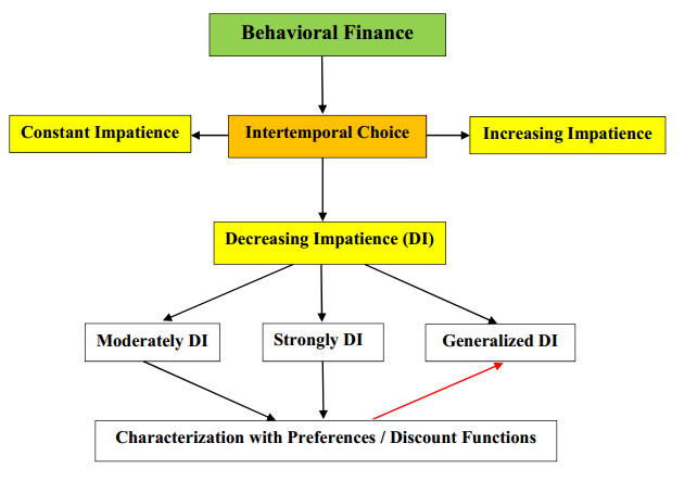
The framework of this paper is behavioral finance and, more specifically, intertemporal choice when individuals exhibit decreasing impatience in their decision-making processes. After characterizing the two main types of decreasing impatience (moderately and strongly decreasing impatience), the main objective of this paper is to generalize these concepts when the criterion of time increase is given by an arbitrary function which describes such increments. In general, the methodology is mathematical calculus but particularly the concept of derivative according to the function which rules the increase of time. The main contribution of this paper is the characterization of this extension of the concept of decreasing impatience by using the aforementioned novel derivative and the well-known Prelec's index.

Keywords:

Citation: Salvador Cruz Rambaud, Fabrizio Maturo, Javier Sánchez García. Generalizing the concept of decreasing impatience[J]. AIMS Mathematics, 2023, 8(4): 7990-7999. doi: 10.3934/math.2023403

Related Papers:

[1]	Qi Xiao, Jin Zhong . Characterizations and properties of hyper-dual Moore-Penrose generalized inverse. AIMS Mathematics, 2024, 9(12): 35125-35150. doi: 10.3934/math.20241670
[2]	Waleed Mohamed Abd-Elhameed, Amr Kamel Amin, Nasr Anwer Zeyada . Some new identities of a type of generalized numbers involving four parameters. AIMS Mathematics, 2022, 7(7): 12962-12980. doi: 10.3934/math.2022718
[3]	Faik Babadağ . A new approach to Jacobsthal, Jacobsthal-Lucas numbers and dual vectors. AIMS Mathematics, 2023, 8(8): 18596-18606. doi: 10.3934/math.2023946
[4]	Changsheng Luo, Jiagui Luo . Complete solutions of the simultaneous Pell equations $(a^2+1)y^2-x^2 = y^2-bz^2 = 1$ . AIMS Mathematics, 2021, 6(9): 9919-9938. doi: 10.3934/math.2021577
[5]	Cencen Dou, Jiagui Luo . Complete solutions of the simultaneous Pell's equations $(a^2+2)x^2-y^2 = 2$ and $x^2-bz^2 = 1$ . AIMS Mathematics, 2023, 8(8): 19353-19373. doi: 10.3934/math.2023987
[6]	Faik Babadağ, Ali Atasoy . A new approach to Leonardo number sequences with the dual vector and dual angle representation. AIMS Mathematics, 2024, 9(6): 14062-14074. doi: 10.3934/math.2024684
[7]	Elahe Mehraban, T. Aaron Gulliver, Salah Mahmoud Boulaaras, Kamyar Hosseini, Evren Hincal . New sequences from the generalized Pell $p-$ numbers and mersenne numbers and their application in cryptography. AIMS Mathematics, 2024, 9(5): 13537-13552. doi: 10.3934/math.2024660
[8]	Bin Zhou, Xiujuan Ma, Fuxiang Ma, Shujie Gao . Robustness analysis of random hyper-networks based on the internal structure of hyper-edges. AIMS Mathematics, 2023, 8(2): 4814-4829. doi: 10.3934/math.2023239
[9]	Waleed Mohamed Abd-Elhameed, Anna Napoli . New formulas of convolved Pell polynomials. AIMS Mathematics, 2024, 9(1): 565-593. doi: 10.3934/math.2024030
[10]	Ümit Tokeşer, Tuğba Mert, Yakup Dündar . Some properties and Vajda theorems of split dual Fibonacci and split dual Lucas octonions. AIMS Mathematics, 2022, 7(5): 8645-8653. doi: 10.3934/math.2022483

Abstract

1. Introduction

Dual numbers were first given by Clifford (1845–1879), and some properties of those were studied in the geometrical investigation, and Kotelnikov ^[1] introduced their first applications. Study applied to line geometry and kinematics dual numbers and dual vectors ^[2]. He demonstrated that the directed lines of Euclidean 3-space and the points of the dual unit sphere in $\mathbb{D}^3$ have a one-to-one relationship. Field theory also relies heavily on these numbers ^[3]. The most intriguing applications of dual numbers in field theory are found in a number of Wald publications ^[4]. Dual numbers have contemporary applications in kinematics, dynamics, computer modeling of rigid bodies, mechanism design, and kinematics ^[5,6,7].

Complex numbers have significant advantages in derivative computations. However, the second derivative computations lost these advantages ^[8]. J. A. Fike developed the hyper-dual numbers to solve this issue ^[9]. These numbers may be used to calculate both the first and second derivatives while maintaining the benefits of the first derivative using complex numbers. Furthermore, it is demonstrated that this numerical approach is appropriate for open kinematic chain robot manipulators, sophisticated software, and airspace system analysis and design ^[10].

In the literature, sequences of integers have an important place. The most famous of these sequences have been demonstrated in several areas of mathematics. These sequences have been researched extensively because of their complex characteristics and deep connections to several fields of mathematics. The Fibonacci and Lucas sequences and their related numbers are of essential importance due to their various applications in biology, physics, statistics, and computer science ^[11,12,13]. Many authors were interested in introducing and investigating several generalizations and modifications of Fibonacci and Lucas sequences. The authors investigated two classes that generalize Fibonacci and Lucas sequences, and they utilized them to compute some radicals in reduced forms. Panwar ^[14] defined the generalized $k$ -Fibonacci sequence as

$\begin{align*} F_{k, n} = pkF_{k, n-1}+qF_{k, n-2}, \end{align*}$

with initial conditions $F_{k, 0} = a$ and $F_{k, 1} = b$ . If $a = 0, k = 2, p = q = b = 1$ , the classic Pell sequence and for $a = b = 2, k = 2, p = q = 1$ , Pell-Lucas sequences appear.

The Pell numbers are the numbers of the following integer sequence:

$0, 1, 2, 5, 12, 29, 70, 169, 408, 985, 2378, ...$

The sequence of Pell numbers, which is denoted by ${P}_n$ is defined as the linear reccurence relation

$\begin{align*} P_n = 2P_{n-1}+P_{n-2} , \quad P_0 = 0, P_1 = 1, \ \ n\ge2. \end{align*}$

The integer sequence of Pell-Lucas numbers denoted by ${Q}_n$ is given by

$2, 2, 6, 14, 34, 82, 198, 478, 1154, 2786, 6726, ...$ ,

with the same reccurence relation

$\begin{align*} Q_n = 2Q_{n-1}+Q_{n-2} , \quad Q_0 = Q_1 = 2, \ \ n\ge2. \end{align*}$

The characteristic equation of these numbers is $x^2-2x-1 = 0$ , with roots $\alpha = 1+\sqrt{2}$ and $\beta = 1-\sqrt{2}$ and the Binet's forms of these sequences are given as^{[15,16,17,18]},

$\begin{equation} P_n = \frac{\alpha^n-\beta^n}{\alpha-\beta} \end{equation}$

(1.1)

and

$\begin{equation} Q_n = \alpha^n+\beta^n. \end{equation}$

(1.2)

The set of dual numbers is defined as

$\begin{equation*} \mathbb{D} = \{d = a+\varepsilon a^{*}\mid a, a^{*}\in \mathbb{R}, \varepsilon ^2 = 0, \varepsilon \neq 0\}. \end{equation*}$

The set of hyper-dual numbers is

$\begin{align*} \widetilde{\mathbb{D}} = \left \{\gamma = \gamma_0+\gamma_1\varepsilon +\gamma_2\varepsilon^* +\gamma_3\varepsilon\varepsilon^* \mid \gamma_0, \gamma_1, \gamma_2, \gamma_3\in \mathbb{R}\right\}, \end{align*}$

or can be rewritten as

$\begin{align*} \widetilde{\mathbb{D}} = \left \{\gamma = d+\varepsilon^*d^* \mid d, d^*\in \mathbb{D}\right\}, \end{align*}$

where $\varepsilon$ , $\varepsilon^*$ and $\varepsilon\varepsilon^*$ are hyper-dual units that satisfy

$\begin{equation*} (\varepsilon)^2 = ({\varepsilon^*})^2 = 0, \; \varepsilon\neq\varepsilon^*\neq0, \; \varepsilon\varepsilon^* = \varepsilon^*\varepsilon. \end{equation*}$

This set forms commutative and associative algebra over both the dual and real numbers ^[8,9,10].

The square root of a hyper-dual number $\gamma$ can be defined by

$\begin{equation} \sqrt{\gamma} = \sqrt{\gamma_{0}}+\frac{\gamma_{1}}{2\sqrt{\gamma_{0}}}\varepsilon+\frac{\gamma_{2}}{2\sqrt{\gamma_{0}}}\varepsilon^*+(\frac{\gamma_{3}}{2\sqrt{\gamma_{0}}}-\frac{\gamma_{1}\gamma_{2}}{4\gamma_{0}\sqrt{\gamma_{0}}})\varepsilon\varepsilon^*. \end{equation}$

(1.3)

A hyper-dual vector is any vector of the form

$\begin{align*} \vec{\gamma} = \vec{\gamma}_{0}+\vec{\gamma}_{1}\varepsilon+\vec{\gamma}_{2}\varepsilon^*+\vec{\gamma}_{3}\varepsilon\varepsilon^*, \end{align*}$

where $\vec{\gamma}_{0}, \vec{\gamma}_{1}, \vec{\gamma}_{2}, \vec{\gamma}_{3}$ are real vectors, this vector can be rewritten as $\vec{\gamma} = \vec{d}+\varepsilon^*\vec{d}^*$ , where $\vec{d}$ and $\vec{d}^*$ are dual vectors. Let $\vec{\gamma}$ and $\vec{\delta}$ be hyper-dual vectors, then their scalar product is defined as

$\begin{align} \langle \vec{\gamma}, \vec{\delta}\rangle_{HD} = &\langle\vec{\gamma}_{0}, \vec{\delta}_{0}\rangle +\left(\langle \vec{\gamma}_{0}, \vec{\delta}_{1}\rangle+\langle \vec{\gamma}_{1}, \vec{\delta}_{0}\rangle\right)\varepsilon+\left(\langle \vec{\gamma}_{0}, \vec{\delta}_{2}\rangle+\langle \vec{\gamma}_{2}, \vec{\delta}_{0}\rangle\right)\varepsilon^*\\[6pt] &+\left(\langle \vec{\gamma}_{0}, \vec{\delta}_{3}\rangle+\langle \vec{\gamma}_{1}, \vec{\delta}_{2}\rangle+\langle \vec{\gamma}_{2}, \vec{\delta}_{1}\rangle+\langle \vec{\gamma}_{3}, \vec{\delta}_{0}\rangle\right) \varepsilon\varepsilon^*, \end{align}$

(1.4)

which continents inner products of real vectors.

Let $f(x_0+ x_1\varepsilon+ x_2\varepsilon^*+ x_3\varepsilon\varepsilon^*)$ be a hyper-dual function, then

$\begin{align} f(x_0+ x_1\varepsilon+ x_2\varepsilon^*+ x_3\varepsilon\varepsilon^*) = f(x_0)+x_1f(x_0)\varepsilon+x_2f'(x_0)\varepsilon^*+(x_3f'(x_0)+x_1x_2f''(x_0))\varepsilon\varepsilon^*. \end{align}$

(1.5)

Suppose $\vec{\gamma}$ , $\vec{\delta}$ and $\Phi$ be unit hyper-dual vectors and hyper-dual angle respectively then by using (1.5) the scalar product can be written as

$\begin{align} \langle\vec{\gamma}, \vec{\delta}\rangle_{HD} & = \cos{\Phi}\\ & = \cos\phi-\varepsilon^* \phi^{\ast }\sin\phi\\ & = (\cos\psi -\varepsilon \psi^{\ast }\sin\psi)-\varepsilon^* \phi^{\ast }(\sin\psi+\varepsilon \psi^{\ast }\cos\psi), \end{align}$

(1.6)

where $\phi$ and $\psi$ are, respectively, dual and real angles.

The norm of a hyper-dual vector $\vec{\gamma}$ is given by

$\begin{align*} \left\| \vec{\gamma}\right\|_{HD} & = \left\| \vec{\gamma}_0\right\|+\frac{\langle \vec{\gamma}_0, \vec{\gamma}_1\rangle }{\left\| \vec{\gamma}_0\right\|}\varepsilon+\frac{\langle \vec{\gamma}_0, \vec{\gamma}_2\rangle }{\left\| \vec{\gamma}_0\right\|} \varepsilon^* +\left(\frac{\langle \vec{\gamma}_0, \vec{\gamma}_3\rangle }{\left\| \vec{\gamma}_0\right\|}+\frac{\langle \vec{\gamma}_1, \vec{\gamma}_2\rangle }{\left\| \vec{\gamma}_0\right\|}-\frac{\langle \vec{\gamma}_0, \vec{\gamma}_1\rangle \langle \vec{\gamma}_0, \vec{\gamma}_2\rangle}{\left\| \vec{\gamma}_0\right\|^3}\right)\varepsilon\varepsilon^*, \end{align*}$

for $\left\| \vec{\gamma}_0\right\|\neq0$ . If $\left\| \vec{\gamma}\right\|_{HD} = 1$ that is $\left\| \vec{\gamma}_0\right\| = 1$ and $\langle \vec{\gamma}_0, \vec{\gamma}_1\rangle = \langle \vec{\gamma}_0, \vec{\gamma}_2\rangle = \langle \vec{\gamma}_0, \vec{\gamma}_3\rangle = \langle \vec{\gamma}_1, \vec{\gamma}_2\rangle = 0$ , then $\vec{\gamma}$ is a unit hyper-dual vector.

In this paper, we introduce the hyper-dual Pell and the hyper-dual Pell-Lucas numbers, which provide a natural generalization of the classical Pell and Pell-Lucas numbers by using the concept of hyper-dual numbers. We investigate some basic properties of these numbers. We also define a new vector and angle, which are called hyper-dual Pell vector and angle. We give properties of these vectors and angles to exert in the geometry of hyper-dual space.

2. Hyper-dual Pell and Hyper-dual Pell-Lucas numbers

In this section, we define the hyper-dual Pell and hyper-dual Pell-Lucas numbers and then demonstrate their fundamental identities and properties.

Definition 2.1. The $n^{th}$ hyper-dual Pell ${\mathrm{HP}}_n$ and hyper-dual Pell-Lucas ${\mathrm{HQ}}_n$ numbers are defined respectively as

$\begin{align} {\mathrm{HP}}_n = \mathrm{P}_n+\mathrm{P}_{n+1}\varepsilon+\mathrm{P}_{n+2}\varepsilon^*+\mathrm{P}_{n+3}\varepsilon\varepsilon^* \end{align}$

(2.1)

and

$\begin{align} \mathrm{HQ}_n = \mathrm{Q}_n+\varepsilon\mathrm{Q}_{n+1}+\varepsilon^*\mathrm{Q}_{n+2}+\varepsilon\varepsilon^*\mathrm{Q}_{n+3}, \end{align}$

(2.2)

where $\mathrm{P}_n$ and $\mathrm{Q}_n$ are $n^{th}$ Pell and Pell-Lucas numbers.

The few hyper-dual Pell and hyper-dual Pell-Lucas numbers are given as

${\mathrm{HP}}_1 = 1+2\varepsilon+5\varepsilon^*+12\varepsilon\varepsilon^*, {\mathrm{HP}}_2 = 2+5\varepsilon+12\varepsilon^*+29\varepsilon\varepsilon^*, ...$

and

${\mathrm{HQ}}_1 = 2+6\varepsilon+14\varepsilon^*+34\varepsilon\varepsilon^*, {\mathrm{HQ}}_2 = 6+14\varepsilon+34\varepsilon^*+82\varepsilon\varepsilon^*, ...$

Theorem 2.1. The Binet-like formulas of the hyper-dual Pell and hyper-dual Pell-Lucas numbers are given, respectively, by

$\begin{align} {\mathrm{HP}}_n = \frac{\varphi^n\;\underline{\varphi}-\psi^n\;\underline{\psi}}{\varphi-\psi} \end{align}$

(2.3)

and

$\begin{align} {\mathrm{HQ}}_n = \varphi^n\;\underline{\varphi}+\psi^n\;\underline{\psi}, \end{align}$

(2.4)

where

$\begin{align} \underline{\varphi} = 1+\varphi\varepsilon+\varphi^{2}\varepsilon^*+\varphi^{3}\varepsilon\varepsilon^*, \; \underline{\psi} = 1+\psi\varepsilon+\psi^{2}\varepsilon^*+\psi^{3}\varepsilon\varepsilon^*. \end{align}$

(2.5)

Proof. From (2.1) and the Binet formula of Pell numbers, we obtain

$\begin{align*} {\mathrm{HP}}_n& = \mathrm{P}_n+\mathrm{P}_{n+1}\varepsilon+\mathrm{P}_{n+2}\varepsilon^*+\mathrm{P}_{n+3}\varepsilon\varepsilon^*\\[6pt] & = \frac{\varphi^n-\psi^n}{\varphi-\psi}+\frac{\varphi^{n+1}-\psi^{n+1}}{\varphi-\psi}\varepsilon+\frac{\varphi^{n+2}-\psi^{n+2}}{\varphi-\psi}\varepsilon^*+\frac{\varphi^{n+3}-\psi^{n+3}}{\varphi-\psi}\varepsilon\varepsilon^*\\[6pt] & = \frac{\varphi^n(1+\varphi\varepsilon+\varphi^{2}\varepsilon^*+\varphi^{3}\varepsilon\varepsilon^*)}{\varphi-\psi}-\frac{\psi^n(1+\psi\varepsilon+\psi^{2}\varepsilon^*+\psi^{3}\varepsilon\varepsilon^*)}{\varphi-\psi} \\[6pt] & = \frac{\varphi^n\; \underline{\varphi}-\psi^n\; \underline{\psi}}{\varphi-\psi}. \end{align*}$

On the other hand, using (2.2) and the Binet formula of Pell-Lucas numbers we obtain

$\begin{align*} {\mathrm{HQ}}_n& = \mathrm{Q}_n+\mathrm{Q}_{n+1}\varepsilon+\mathrm{Q}_{n+2}\varepsilon^*+\mathrm{Q}_{n+3}\varepsilon\varepsilon^*\\[6pt] & = \left( \varphi^n+\psi^n \right)+\left( \varphi^{n+1}+\psi^{n+1} \right)\varepsilon+\left( \varphi^{n+2}+\psi^{n+2} \right)\varepsilon^*+\left( \varphi^{n+3}+\psi^{n+3} \right)\varepsilon\varepsilon^*\\[6pt] & = \varphi^n(1+\varphi\varepsilon+\varphi^{2}\varepsilon^*+\varphi^{3}\varepsilon\varepsilon^*)+\psi^n(1+\psi\varepsilon+\psi^{2}\varepsilon^*+\psi^{3}\varepsilon\varepsilon^*) \\[6pt] & = \varphi^n\; \underline{\varphi}+\psi^n\; \underline{\psi}. \end{align*}$

□ The proof is completed.

Theorem 2.2. (Vajda-like identities) For non-negative integers m, n, and r, we have

$\begin{align*} &{\mathrm{HP}}_{m}{\mathrm{HP}}_{n}-{\mathrm{HP}}_{m-r}{\mathrm{HP}}_{n+r} = (-1)^{n+1}\mathrm{P}_{m-n-r}\mathrm{P}_{r}\left( 1+2\varepsilon+6\varepsilon^*+12\varepsilon\varepsilon^* \right), \\[6pt] &{\mathrm{HQ}}_{m}{\mathrm{HQ}}_{n}-{\mathrm{HQ}}_{m-r}{\mathrm{HQ}}_{n+r} = (-1)^{n}\; \mathrm{Q}_{m-n}-(-1)^{n+r}\; \mathrm{Q}_{m-n-2r}\; \left( 1+2\varepsilon+6\varepsilon^*+12\varepsilon\varepsilon^* \right). \end{align*}$

Proof. By using the Binet-like formula of hyper-dual Pell numbers, we obtain

$\begin{align*} {\mathrm{HP}}_{m}{\mathrm{HP}}_{n}-{\mathrm{HP}}_{m-r}{\mathrm{HP}}_{n+r}& = \left(\frac{\; \varphi^{m}\underline{\varphi}-\; \psi^{m}\underline{\psi}}{\varphi-\psi}\right)\left(\frac{\; \varphi^{n}\underline{\varphi}-\; \psi^{n}\underline{\psi}}{\varphi-\psi}\right) -\left(\frac{\; \varphi^{m-r}\underline{\varphi}-\; \psi^{m-r}\underline{\psi}}{\varphi-\psi}\right)\left(\frac{\; \varphi^{n+r}\underline{\varphi}-\; \psi^{n+r}\underline{\psi}}{\varphi-\psi}\right)\\[6pt] & = \frac{(\varphi^{r}-\psi^{r})(\varphi^{n}\psi^{m-r}-\psi^{n}\varphi^{m-r})}{(\varphi-\psi)^2}\underline{\varphi}\; \underline{\psi}\\[6pt] & = -\frac{(\varphi^{m-n-r}-\psi^{m-n-r})(\varphi^{r}-\psi^{r})}{(\varphi-\psi)^2}\underline{\varphi}\; \underline{\psi}, \end{align*}$

and by using (1.1), we obtain

$\begin{equation*} {\mathrm{HP}}_{m}{\mathrm{HP}}_{n}-{\mathrm{HP}}_{m-r}{\mathrm{HP}}_{n+r} = (-1)^{n+1}\mathrm{P}_{m-n-r}\mathrm{P}_{r}\left( 1+2\varepsilon+6\varepsilon^*+12\varepsilon\varepsilon^* \right). \end{equation*}$

Similarly for hyper-dual Pell-Lucas numbers, we can obtain

$\begin{align*} {\mathrm{HQ}}_{m}{\mathrm{HQ}}_{n}-{\mathrm{HQ}}_{m-r}{\mathrm{HQ}}_{n+r}& = \left(\; \varphi^{m}\underline{\varphi}+\; \psi^{m}\underline{\psi}\right)\left(\; \varphi^{n}\underline{\varphi}+\; \psi^{n}\underline{\psi}\right)\\&\quad-\left(\; \varphi^{m-r}\underline{\varphi}+\; \psi^{m-r}\underline{\psi}\right)\left(\; \varphi^{n+r}\underline{\varphi}+\; \psi^{n+r}\underline{\psi}\right) \\& = \underline{\varphi}\; \underline{\psi}\left(\varphi^{m-n}+\psi^{m-n}-\varphi^{m-n-2r}-\psi^{m-n-2r}\right). \end{align*}$

Using (1.2) and (2.5),

$\begin{align*} {\mathrm{HQ}}_{m}{\mathrm{HQ}}_{n}-{\mathrm{HQ}}_{m-r}{\mathrm{HQ}}_{n+r} = (-1)^{n}\; \mathrm{Q}_{m-n}-(-1)^{n+r}\; \mathrm{Q}_{m-n-2r}\; \left( 1+2\varepsilon+6\varepsilon^*+12\varepsilon\varepsilon^* \right). \end{align*}$

Thus, we obtain the desired results. □

Theorem 2.3. (Catalan-like identities) For non negative integers n and r, with $n\ge r$ , we have

$\begin{align*} &{\mathrm{HP}}_{n-r}{\mathrm{HP}}_{n+r}-{{\mathrm{HP}}}_{n}^2 = (-1)^{n-r}\mathrm{P}_{r}^{2}\left( 1+2\varepsilon+6\varepsilon^*+12\varepsilon\varepsilon^* \right), \\[6pt] &{\mathrm{HQ}}_{n-r}{\mathrm{HQ}}_{n+r}-{\mathrm{HQ}}_{n}^2 = 8(-1)^{n-r}\; \mathrm{P}_{r}^{2}\; \left( 1+2\varepsilon+6\varepsilon^*+12\varepsilon\varepsilon^* \right). \end{align*}$

Proof. From (2.3), we obtain

$\begin{align*} {\mathrm{HP}}_{n-r}{\mathrm{HP}}_{n+r}-{\mathrm{HP}}_{n}^2& = \left(\frac{\; \varphi^{n-r}\underline{\varphi}-\; \psi^{n-r}\underline{\psi}}{\varphi-\psi}\right)\left(\frac{\; \varphi^{n+r}\underline{\varphi}-\; \psi^{n+r}\underline{\psi}}{\varphi-\psi}\right)-\left(\frac{\; \varphi^n\underline{\varphi}-\; \psi^n\underline{\psi}}{\varphi-\psi}\right)^2\\[6pt] & = \frac{\varphi^{n}\psi^{n}}{8}\; \underline{\varphi}\; \underline{\psi}\left(2-\psi^{r}\varphi^{-r}-\psi^{-r}\varphi^{r}\right)\\[6pt] & = (-1)^{n-r}\; \underline{\varphi}\; \underline{\psi}\left(\frac{\varphi^{r}-\psi^{r}}{\varphi-\psi}\right)^{2}, \end{align*}$

and by using (1.1) and (2.5), we will have

$\begin{equation*} {\mathrm{HP}}_{n-r}{\mathrm{HP}}_{n+r}-{\mathrm{HP}}_{n}^2 = (-1)^{n-r}\mathrm{P}_{r}^{2}\left( 1+2\varepsilon+6\varepsilon^*+12\varepsilon\varepsilon^* \right). \end{equation*}$

On the other hand, from (2.4) and (2.5) we obtain

$\begin{align*} {\mathrm{HQ}}_{n-r}{\mathrm{HQ}}_{n+r}-{\mathrm{HQ}}_{n}^2& = \left(\; \varphi^{n-r}\underline{\varphi}+\; \psi^{n-r}\underline{\psi}\right)\left(\; \varphi^{n+r}\underline{\varphi}+\; \psi^{n+r}\underline{\psi}\right)-\left(\; \varphi^n\underline{\varphi}+\; \psi^n\underline{\psi}\right)^2 \\& = \underline{\varphi}\; \underline{\psi}\left(\varphi^{n-r}\psi^{n+r}+\varphi^{n+r}\psi^{n-r}-2\psi^{n}\varphi^{n}\right)\\ & = 8(-1)^{n-r}\; \underline{\varphi}\; \underline{\psi}\left(\frac{\varphi^{r}-\psi^{r}}{\varphi-\psi}\right)^{2}\\ & = 8(-1)^{n-r}\; \mathrm{P}_{r}^{2}\; \left( 1+2\varepsilon+6\varepsilon^*+12\varepsilon\varepsilon^* \right). \end{align*}$

□

Corollary 2.1. (Cassini-like identities) For non-negative integer n, we have

$\begin{align*} &\mathrm{HP}_{n-1}\; \mathrm{HP}_{n+1}-\mathrm{HP}_{n}^2 = (-1)^{n-1}\left( 1+2\varepsilon+6\varepsilon^*+12\varepsilon\varepsilon^* \right), \\[6pt] &\mathrm{HQ}_{n-1}\; \mathrm{HQ}_{n+1}- \mathrm{HQ}_{n}^2 = 8(-1)^{n-1}\left( 1+2\varepsilon+6\varepsilon^*+12\varepsilon\varepsilon^* \right). \end{align*}$

Proof. We can get the result by taking $r = 1$ in Theorem 2.3. □

Theorem 2.4. (d'Ocagne-like identities) For non-negative integers n and m,

$\begin{align*} &\mathrm{HP}_{m+1}\; \mathrm{HP}_{n}-\mathrm{HP}_{m}\; \mathrm{HP}_{n+1} = \left( -1 \right)^{m}\mathrm{P}_{n-m}\left( 1+2\varepsilon+6\varepsilon^*+12\varepsilon\varepsilon^* \right), \\[6pt] &\mathrm{HQ}_{m+1}\; \mathrm{HQ}_{n}-\mathrm{HQ}_{m}\; \mathrm{HQ}_{n+1} = 8\left( -1 \right)^{n}\mathrm{P}_{m-n}\left( 1+2\varepsilon+6\varepsilon^*+12\varepsilon\varepsilon^* \right). \end{align*}$

Proof. Using (1.1), (2.3), and (2.5), we have

$\begin{align*} \mathrm{HP}_{m+1}\; \mathrm{HP}_{n}-\mathrm{HP}_{m}\; \mathrm{HP}_{n+1}& = \left(\frac{\; \varphi^{m+1}\underline{\varphi}-\; \psi^{m+1}\underline{\psi}}{\varphi-\psi}\right)\left(\frac{\; \varphi^{n}\underline{\varphi}-\; \psi^{n}\underline{\psi}}{\varphi-\psi}\right)\\ &\quad-\left(\frac{\; \varphi^{m}\underline{\varphi}-\; \psi^{m}\underline{\psi}}{\varphi-\psi}\right)\left(\frac{\; \varphi^{n+1}\underline{\varphi}-\; \psi^{n+1}\underline{\psi}}{\varphi-\psi}\right)\\ & = (\varphi-\psi)(\varphi^{n}\psi^{m}-\varphi^{m}\psi^{n}) \underline{\varphi}\; \underline{\psi} \\ & = \left( -1 \right)^{m}\mathrm{P}_{n-m}\left( 1+2\varepsilon+6\varepsilon^*+12\varepsilon\varepsilon^* \right). \end{align*}$

Using (1.2), (2.4) and (2.5), we have

$\begin{align*} \mathrm{HQ}_{m+1}\; \mathrm{HQ}_{n}-\mathrm{HQ}_{m}\; \mathrm{HQ}_{n+1} = 8\left( -1 \right)^{n}\mathrm{P}_{m-n}\left( 1+2\varepsilon+6\varepsilon^*+12\varepsilon\varepsilon^* \right). \end{align*}$

□

3. Hyper dual Pell vectors and angle

In this section, we introduce hyper-dual Pell vectors and hyper-dual Pell angle. We will give geometric properties of them.

Definition 3.1. The $n^{th}$ hyper-dual Pell vector is defined as

$\begin{align*} \overrightarrow{{\mathrm{HP}}}_n = \vec{\mathrm{P}}_n+\vec{\mathrm{P}}_{n+1}\varepsilon+\vec{\mathrm{P}}_{n+2}\varepsilon^*+\vec{\mathrm{P}}_{n+3}\varepsilon\varepsilon^*, \end{align*}$

where $\vec{\mathrm{P}}_{n} = (\mathrm{P}_n, \mathrm{P}_{n+1}, \mathrm{P}_{n+2})$ is a real Pell vector. The hyper-dual Pell vector $\overrightarrow{\mathrm{HP}}_n$ can be rewritten in terms of dual Pell vectors $\vec{\mathbb{P}}_n$ and $\vec{\mathbb{P}} ^*_{n}$ as

$\begin{align*} \nonumber \overrightarrow{\mathrm{HP}}_n & = (\vec{\mathrm{P}}_n+\vec{\mathrm{P}}_{n+1}\varepsilon)+(\vec{\mathrm{P}}_{n+2}+\vec{\mathrm{P}}_{n+3}\varepsilon)\varepsilon^* \\ & = \vec{\mathbb{P}}_n+\varepsilon^*\vec{\mathbb{P}} ^*_{n}. \end{align*}$

Theorem 3.1. The scalar product of hyper-dual Pell vectors $\overrightarrow{{\mathrm{HP}}}_n$ and $\overrightarrow{{\mathrm{HP}}}_m$ is

$\begin{align} \langle \overrightarrow{\mathrm{HP}}_n, \overrightarrow{\mathrm{HP}}_m \rangle = &\frac{7\mathrm{Q}_{n+m+2}}{8}-\frac{(-1)^{m}\mathrm{Q}_{n-m}}{8} +(\frac{7\mathrm{Q}_{n+m+3}}{4}-\frac{(-1)^{m}\mathrm{Q}_{n-m}}{4})\varepsilon \\ &+(\frac{7\mathrm{Q}_{n+m+4}}{4}-\frac{3(-1)^{m}\mathrm{Q}_{n-m}}{4})\varepsilon^* +(\frac{7\mathrm{Q}_{n+m+5}}{2}-\frac{3(-1)^{m}\mathrm{Q}_{n-m}}{2})\varepsilon\varepsilon^*. \end{align}$

(3.1)

Proof. By using (1.4), we can write

$\begin{align} \langle \overrightarrow{\mathrm{HP}}_n, \overrightarrow{\mathrm{HP}}_{m}\rangle = &\langle\vec{\mathrm{P}}_{n}, \vec{\mathrm{P}}_{m}\rangle +\left(\langle \vec{\mathrm{P}}_{n}, \vec{\mathrm{P}}_{m+1}\rangle+\langle \vec{\mathrm{P}}_{n+1}, \vec{\mathrm{P}}_{m}\rangle\right)\varepsilon+\left(\langle\vec{\mathrm{P}}_{n}, \vec{\mathrm{P}}_{m+2}\rangle+\langle \vec{\mathrm{P}}_{n+2}, \vec{\mathrm{P}}_{m}\rangle\right)\varepsilon^*\\[6pt] &+\left(\langle \vec{\mathrm{P}}_{n}, \vec{\mathrm{P}}_{m+3}\rangle+\langle \vec{\mathrm{P}}_{n+1}, \vec{\mathrm{P}}_{m+2}\rangle+\langle \vec{\mathrm{P}}_{n+2}, \vec{\mathrm{P}}_{m+1}\rangle+\langle \vec{\mathrm{P}}_{n+3}, \vec{\mathrm{P}}_{m}\rangle\right) \varepsilon\varepsilon^*. \end{align}$

(3.2)

Now we calculate the above inner products for real Pell vectors $\vec{\mathrm{P}}_{n}$ and $\vec{\mathrm{P}}_{m}$ by using Binet's formula of Pell numbers as

$\begin{align*} \langle \vec{\mathrm{P}}_n, \vec{\mathrm{P}}_{m}\rangle& = \mathrm{P}_{n}\mathrm{P}_{m}+\mathrm{P}_{n+1}\mathrm{P}_{m+1}+ \mathrm{P}_{n+2}\mathrm{P}_{m+2} \\ & = \left(\frac{\varphi^{n}-\psi^{n}}{\varphi-\psi}\right)\left(\frac{\varphi^{m}-\psi^{m}}{\varphi-\psi}\right)+\left(\frac{\varphi^{n+1}-\psi^{n+1}}{\varphi-\psi}\right)\left(\frac{\varphi^{m+1}-\psi^{m+1}}{\varphi-\psi}\right) +\left(\frac{\varphi^{n+2}-\psi^{n+2}}{\varphi-\psi}\right)\left(\frac{\varphi^{m+2}-\psi^{m+2}}{\varphi-\psi}\right)\\ & = \frac{\varphi^{n+m}+\psi^{n+m}}{(\varphi-\psi)^2}+\frac{\varphi^{n+m+2}+\psi^{n+m+2}}{(\varphi-\psi)^2} +\frac{\varphi^{n+m+4}+\psi^{n+m+4}}{(\varphi-\psi)^2}-\frac{\left( \varphi^{n}\psi^{m}+\varphi^{m}\psi^{n} \right)\varphi^{-m}\psi^{-m}}{(\varphi-\psi)^2\; \varphi^{-m}\psi^{-m}} \\ & = \frac{1}{8}\left( \mathrm{Q}_{n+m}+\mathrm{Q}_{n+m+2}+\mathrm{Q}_{n+m+4}+(-1)^{m}\mathrm{Q}_{n-m} \right)\\ & = \frac{7\mathrm{Q}_{n+m+2}}{8}-\frac{(-1)^{m}\mathrm{Q}_{n-m}}{8}. \end{align*}$

□ Similarly,

$\begin{align*} \langle \vec{\mathrm{P}}_n, \vec{\mathrm{P}}_{m+1} \rangle& = \frac{7\mathrm{Q}_{n+m+3}}{8}+\frac{(-1)^{m}\mathrm{Q}_{n-m-1}}{8}, \\ \langle \vec{\mathrm{P}}_{n+1}, \vec{\mathrm{P}}_{m} \rangle& = \frac{7\mathrm{Q}_{n+m+3}}{8}-\frac{(-1)^{m}\mathrm{Q}_{n-m+1}}{8}, \\ \langle \vec{\mathrm{P}}_{n}, \vec{\mathrm{P}}_{m+2} \rangle& = \frac{7\mathrm{Q}_{n+m+4}}{8}-\frac{(-1)^{m}\mathrm{Q}_{n-m-2}}{8}, \\ \langle \vec{\mathrm{P}}_{n+2}, \vec{\mathrm{P}}_{m} \rangle& = \frac{7\mathrm{Q}_{n+m+4}}{8}-\frac{(-1)^{m}\mathrm{Q}_{n-m+2}}{8}, \\ \langle \vec{\mathrm{P}}_{n}, \vec{\mathrm{P}}_{m+3} \rangle& = \frac{7\mathrm{Q}_{n+m+5}}{8}+\frac{(-1)^{m}\mathrm{Q}_{n-m-3}}{8}, \\ \langle \vec{\mathrm{P}}_{n+1}, \vec{\mathrm{P}}_{m+2} \rangle& = \frac{7\mathrm{Q}_{n+m+5}}{8}-\frac{(-1)^{m}\mathrm{Q}_{n-m-1}}{8}, \\ \langle \vec{\mathrm{P}}_{n+2}, \vec{\mathrm{P}}_{m+1} \rangle& = \frac{7\mathrm{Q}_{n+m+5}}{8}+\frac{(-1)^{m}\mathrm{Q}_{n-m+1}}{8}, \\ \langle \vec{\mathrm{P}}_{n+3}, \vec{\mathrm{P}}_{m} \rangle& = \frac{7\mathrm{Q}_{n+m+5}}{8}-\frac{(-1)^{m}\mathrm{Q}_{n-m+3}}{8}. \end{align*}$

By substituting these equalities in (3.2), we obtain the result.

Example 3.1. Let $\overrightarrow{{\mathrm{HP}}}_1 = (1, 2, 5)+(2, 5, 12)\varepsilon+(5, 12, 29)\varepsilon^*+(12, 29, 70)\varepsilon\varepsilon^*$ and $\overrightarrow{{\mathrm{HP}}}_0 = (0, 1, 2)+(1, 2, 5)\varepsilon+(2, 5, 12)\varepsilon^*+(5, 12, 29)\varepsilon\varepsilon^*$ be the hyper-dual Pell vectors. The scalar product of $\overrightarrow{{\mathrm{HP}}}_1$ and $\overrightarrow{{\mathrm{HP}}}_0$ are

$\begin{align*} \langle \overrightarrow{\mathrm{HP}}_1, \overrightarrow{\mathrm{HP}}_0 \rangle & = \frac{7\mathrm{Q}_{3}-Q_1}{8} +\frac{7\mathrm{Q}_{4}-Q_1}{4}\varepsilon +\frac{7\mathrm{Q}_{5}-3Q_1}{4}\varepsilon^* +\frac{7\mathrm{Q}_{6}-3Q_1}{2}\varepsilon\varepsilon^*\\ & = 12+59\varepsilon+142\varepsilon^*+690\varepsilon\varepsilon^*. \end{align*}$

By the other hand

$\begin{align*} \langle \overrightarrow{\mathrm{HP}}_1, \overrightarrow{\mathrm{HP}}_{0}\rangle \nonumber & = \langle\vec{\mathrm{P}}_{1}, \vec{\mathrm{P}}_{0}\rangle +\left(\langle \vec{\mathrm{P}}_{1}, \vec{\mathrm{P}}_{1}\rangle+\langle \vec{\mathrm{P}}_{2}, \vec{\mathrm{P}}_{0}\rangle\right)\varepsilon+\left(\langle\vec{\mathrm{P}}_{1}, \vec{\mathrm{P}}_{2}\rangle+\langle \vec{\mathrm{P}}_{3}, \vec{\mathrm{P}}_{0}\rangle\right)\varepsilon^*\\[6pt] &\quad+\left(\langle \vec{\mathrm{P}}_{1}, \vec{\mathrm{P}}_{3}\rangle+\langle \vec{\mathrm{P}}_{2}, \vec{\mathrm{P}}_{2}\rangle+\langle \vec{\mathrm{P}}_{3}, \vec{\mathrm{P}}_{1}\rangle+\langle \vec{\mathrm{P}}_{4}, \vec{\mathrm{P}}_{0}\rangle\right) \varepsilon\varepsilon^*\\ & = 12+(30+29)\varepsilon+(72+70)\varepsilon^*+(174+173+174+169)\varepsilon\varepsilon^*\\ & = 12+59\varepsilon+142\varepsilon^*+690\varepsilon\varepsilon^*. \end{align*}$

The results are the same as we expected.

Corollary 3.1. The norm of $\overrightarrow{{\mathrm{HP}}}_n$ is

$\begin{align} \| \overrightarrow{\mathrm{HP}}_n \|^2 = \langle \overrightarrow{\mathrm{HP}}_n, \overrightarrow{\mathrm{HP}}_n \rangle = &\frac{7\mathrm{Q}_{2n+2}}{8}-\frac{(-1)^{n}}{4} +(\frac{7\mathrm{Q}_{2n+3}}{4}-\frac{(-1)^{n}}{2})\varepsilon \\&+(\frac{7\mathrm{Q}_{2n+4}}{4}-\frac{3(-1)^{n}}{2})\varepsilon^* +(\frac{7\mathrm{Q}_{2n+5}}{2}-3(-1)^{n}\mathrm)\varepsilon\varepsilon^*. \end{align}$

(3.3)

Proof. The proof is clear from taking $m = n$ in (3.1). □

Example 3.2. Find the norm of $\overrightarrow{{\mathrm{HP}}}_1 = (1, 2, 5)+(2, 5, 12)\varepsilon+(5, 12, 29)\varepsilon^*+(12, 29, 70)\varepsilon\varepsilon^*$ .

If we take $n = 1$ in (3.3) and use (1.3), then we will get

$\begin{align*} \| \overrightarrow{\mathrm{HP}}_1 \| & = \sqrt{\frac{7\mathrm{Q}_{4}}{8}+\frac{1}{4} +(\frac{7\mathrm{Q}_{5}}{4}+\frac{1}{2})\varepsilon +(\frac{7\mathrm{Q}_{6}}{4}+\frac{3}{2})\varepsilon^* +(\frac{7\mathrm{Q}_{7}}{2}+3\mathrm)\varepsilon\varepsilon^*}\\ & = \sqrt{30+144\varepsilon+348\varepsilon^*+1676\varepsilon\varepsilon^*}\\ & = \sqrt{30}+\frac{72}{\sqrt{30}}\varepsilon+\frac{174}{\sqrt{30}}\varepsilon^*+\frac{734}{5\sqrt{30}}\varepsilon\varepsilon^*. \end{align*}$

From (1.6) and (3.1), the following cases can be given for the scalar product of hyper-dual Pell vectors $\overrightarrow{\mathrm{HP}}_n$ and $\overrightarrow{\mathrm{HP}}_m$ .

Case 3.1. Assume that $\cos\phi = 0$ and $\phi^{\ast }\neq 0$ , then $\psi = \frac{\pi}{2}$ , $\psi^* = 0$ , therefore

$\begin{align*} \langle \overrightarrow{\mathrm{HP}}_n, \overrightarrow{\mathrm{HP}}_m \rangle = -\varepsilon^* \phi^*& = (\frac{7\mathrm{Q}_{m+n+4}}{4}-\frac{3(-1)^{m}\mathrm{Q}_{n-m}}{4})\varepsilon^*+(\frac{7\mathrm{Q}_{m+n+5}}{2}-\frac{3(-1)^{m}\mathrm{Q}_{n-m}}{2}\mathrm)\varepsilon\varepsilon^*, \end{align*}$

then, we get

$\begin{equation*} \phi^* = \left( -1 \right)^{m} \left( \frac{3}{2}+ \varepsilon\right)-\frac{7}{4}\left( \mathrm{Q}_{m+n+4}+2\; \varepsilon\; \mathrm{Q}_{m+n+5}\right) \end{equation*}$

and corresponding dual lines $\mathrm{}{d}_1$ and ${d}_2$ are perpendicular such that they do not intersect each other; see Figure 1.

Figure 1. Geometric representation of hyper-dual angle between the directed dual lines

${d}_1$ and

${d}_2$ .

DownLoad: Full-Size Img PowerPoint

Case 3.2. Assume that $\phi^{\ast } = 0$ and $\phi\neq0$ , then we obtain

$\begin{align*} \langle \overrightarrow{\mathrm{HP}}_n, \overrightarrow{\mathrm{HP}}_m \rangle = \cos\phi& = \left( \frac{7\mathrm{Q}_{m+n+2}}{8}-\frac{(-1)^{m}\mathrm{Q}_{n-m}}{8} \right)+\left( \frac{7\mathrm{Q}_{m+n+3}}{4}-\frac{(-1)^{m}\mathrm{Q}_{n-m}}{4} \right)\varepsilon, \end{align*}$

therefore

$\begin{equation*} \phi = \arccos\left(\left( \frac{7\mathrm{Q}_{m+n+2}}{8}-\frac{(-1)^{m}{Q}_{n-m}}{8} \right)+\left( \frac{7\mathrm{Q}_{m+n+3}}{4}-\frac{(-1)^{m}{Q}_{n-m}}{4} \right)\varepsilon\right), \end{equation*}$

and corresponding dual lines ${d}_1$ and ${d}_2$ intersect each other; see Figure 2.

Figure 2. Intersection of dual lines

${d}_1$ and

${d}_2$ .

DownLoad: Full-Size Img PowerPoint

Case 3.3. Assume that $\cos\phi = 0$ and $\phi^* = 0$ , then $\psi = \frac{\pi}{2}$ and $\psi^{\ast } = 0$ , therefore

$\begin{align*} \langle \overrightarrow{\mathrm{HP}}_n, \overrightarrow{\mathrm{HP}}_m \rangle & = 0, \end{align*}$

and dual lines ${d}_1$ and ${d}_2$ intersect each other at a right angle; see Figure 3.

Figure 3. Perpendicular intersection of dual lines

${d}_1$ and

${d}_2$ .

DownLoad: Full-Size Img PowerPoint

Case 3.4. Assume that $\phi = 0$ and $\phi^* = 0$ , then

$\begin{align*} \langle \overrightarrow{\mathrm{HP}}_n, \overrightarrow{\mathrm{HP}}_m \rangle & = 1, \end{align*}$

in this case corresponding dual lines ${d}_1$ and ${d}_2$ are parallel; see Figure 4.

Figure 4. Parallel of dual lines

${d}_1$ and

${d}_2$ .

DownLoad: Full-Size Img PowerPoint

4. Conclusions

In the present study, we introduce two families of hyper-dual numbers with components containing Pell and the Pell-Lucas numbers. First, we define hyper-dual Pell and Pell-Lucas numbers. Afterwards, by means of the Binet's formulas of Pell and Pell-Lucas numbers, we investigate identities such as the Binet-like formulas, Vajda-like, Catalan-like, Cassini-like, and d'Ocagne-like identities. After that, we define hyper-dual Pell vector and angle with some properties and geometric applications related to them. In the future it would be valuable to replicate a similar exploration and development of our findings on hyper-dual numbers with Pell and Pell-Lucas numbers. These results can trigger further research on the subjects of the hyper-dual numbers, vector, and angle to carry out in the geometry of dual and hyper-dual space.

Author contributions

Faik Babadağ and Ali Atasoy: Conceptualization, writing-original draft, writing-review, editing. All authors have read and approved the final version of the manuscript for publication.

Conflict of interest

The authors declare that they have no conflict of interest.

References

[1]	S. Cruz Rambaud, B. Torrecillas Jover, An extension of the concept of derivative: Its application to intertemporal choice, Mathematics, 8 (2020), 696. https://doi.org/10.3390/math8050696 doi: 10.3390/math8050696
[2]	S. Cruz Rambaud, I. González Fernández, A measure of inconsistencies in intertemporal choice, PloS ONE, 14 (2019), e0224242. https://doi.org/10.1371/journal.pone.0224242 doi: 10.1371/journal.pone.0224242
[3]	S. Cruz Rambaud, I. González Fernández, A new approach to intertemporal choice: The delay function, Symmetry, 12 (2020), 807. https://doi.org/10.3390/sym12050807 doi: 10.3390/sym12050807
[4]	S. Cruz Rambaud, I. González Fernández, V. Ventre, Modeling the inconsistency in intertemporal choice: The generalized Weibull discount function and its extension, Ann. Financ., 14 (2018), 415–426. https://doi.org/10.1007/s10436-018-0318-3 doi: 10.1007/s10436-018-0318-3
[5]	S. Cruz Rambaud, M. J. Muñoz Torrecillas, A generalization of the $q$ -exponential discounting function, Phys. A Stat. Mech. Appl., 392 (2013), 3045–3050. https://doi.org/10.1016/j.physa.2013.03.009 doi: 10.1016/j.physa.2013.03.009
[6]	S. Cruz Rambaud, M. J. Muñoz Torrecillas, T. Takahashi, Observed and normative discount functions in addiction and other diseases, Front. Pharmacol., 8 (2017), 416. https://doi.org/10.3389/fphar.2017.00416 doi: 10.3389/fphar.2017.00416
[7]	S. Cruz Rambaud, V. Ventre, Deforming time in a nonadditive discount function, Int. J. Intell. Syst., 32 (2017), 467–480. https://doi.org/10.1002/int.21842 doi: 10.1002/int.21842
[8]	L. S. dos Santos, A. S. Martinez, Inconsistency and subjective time dilation perception in intertemporal decision making, Front. Appl. Math. Stat., 4 (2018), 54. https://doi.org/10.3389/fams.2018.00054 doi: 10.3389/fams.2018.00054
[9]	P. C. Fishburn, A. Rubinstein, Time preference, Int. Econ. Rev., 23 (1982), 677–694. https://doi.org/10.2307/2526382 doi: 10.2307/2526382
[10]	J. M. Karpoff, The relation between price changes and trading volume: A survey, The Journal of Financial and Quantitative Analysis, 22 (1987), 109–126. https://doi.org/10.2307/2330874 doi: 10.2307/2330874
[11]	G. Loewenstein, D. Prelec, Anomalies in intertemporal choice: Evidence and an interpretation, The Quarterly Journal of Economics, 107 (1992), 573–597. https://doi.org/10.2307/2118482 doi: 10.2307/2118482
[12]	G. Loewenstein, R. H. Thaler, Anomalies: Intertemporal choice, J. Econ. Perspect., 3 (1989), 181–193. https://doi.org/10.1257/jep.3.4.181 doi: 10.1257/jep.3.4.181
[13]	D. Prelec, Decreasing impatience: A criterion for non-stationary time preference and "hyperbolic" discounting, Scand. J. Econ., 106 (2004), 511–532. https://doi.org/10.1111/j.0347-0520.2004.00375.x doi: 10.1111/j.0347-0520.2004.00375.x
[14]	H. Rachlin, Notes on discounting, J. Exp. Anal. Behav., 85 (2006), 425–435. https://doi.org/10.1901/jeab.2006.85-05 doi: 10.1901/jeab.2006.85-05
[15]	D. Read, Intertemporal Choice. Working Paper LSEOR 03.58. London School of Economics and Political Science, 2003.
[16]	P. H. M. P. Roelofsma, D. Read, Intransitive intertemporal choice, J. Behav. Decis. Making, 13 (2000), 161–177. https://doi.org/10.1002/(SICI)1099-0771(200004/06)13:2<161::AID-BDM348>3.0.CO;2-P doi: 10.1002/(SICI)1099-0771(200004/06)13:2<161::AID-BDM348>3.0.CO;2-P
[17]	K. I. M. Rohde, Measuring decreasing and increasing impatience, Manage. Sci., 65 (2019), 1700–1716. https://doi.org/10.1287/mnsc.2017.3015 doi: 10.1287/mnsc.2017.3015
[18]	P. A. Samuelson, A note on measurement of utility, Rev. Econ. Stud., 4 (1937), 155–161. https://doi.org/10.2307/2967612 doi: 10.2307/2967612
[19]	S. S. Stevens, On the psychophysical law, Psychol. Rev., 64 (1957), 153–181. https://doi.org/10.1037/h0046162 doi: 10.1037/h0046162
[20]	T. Takahashi, A comparison of intertemporal choices for oneself versus someone else based on Tsallis' statistics, Phys. A Stat. Mech. Appl., 385 (2007), 637–644. https://doi.org/10.1016/j.physa.2007.07.020 doi: 10.1016/j.physa.2007.07.020
[21]	T. Takahashi, H. Oono, M. H. B. Radford, Empirical estimation of consistency parameter in intertemporal choice based on Tsallis' statistics, Phys. A Stat. Mech. Appl., 381 (2007), 338–342. https://doi.org/10.1016/j.physa.2007.03.038 doi: 10.1016/j.physa.2007.03.038
[22]	T. Takahashi, H. Oono, M. H. B. Radford, Psychophysics of time perception and intertemporal choice models, Phys. A Stat. Mech. Appl., 387 (2008), 2066–2074, https://doi.org/10.1016/j.physa.2007.11.047 doi: 10.1016/j.physa.2007.11.047

Reader Comments

Your name:*

Email:*
© 2023 the Author(s), licensee AIMS Press. This is an open access article distributed under the terms of the Creative Commons Attribution License (http://creativecommons.org/licenses/by/4.0)

通讯作者: 陈斌, bchen63@163.com

1.
沈阳化工大学材料科学与工程学院沈阳 110142

AIMS Mathematics

1.8 3.4

Metrics

Article views(1402) PDF downloads(57) Cited by(0)

Preview PDF

Download XML

Export Citation

Article outline

Show full outline

AIMS Mathematics

Generalizing the concept of decreasing impatience

Related Papers:

Abstract

1. Introduction

2. Hyper-dual Pell and Hyper-dual Pell-Lucas numbers

3. Hyper dual Pell vectors and angle

4. Conclusions

Author contributions

Conflict of interest

References

Reader Comments

通讯作者: 陈斌, bchen63@163.com

Metrics

Figures and Tables

Other Articles By Authors

Catalog

Abstract

1. Introduction

2. Hyper-dual Pell and Hyper-dual Pell-Lucas numbers

3. Hyper dual Pell vectors and angle

4. Conclusions

Author contributions

Conflict of interest

References

AIMS Mathematics

Generalizing the concept of decreasing impatience

Related Papers:

Abstract

1. Introduction

2. Hyper-dual Pell and Hyper-dual Pell-Lucas numbers

3. Hyper dual Pell vectors and angle

4. Conclusions

Author contributions

Conflict of interest

References

Reader Comments

通讯作者: 陈斌, bchen63@163.com

Metrics

Figures and Tables

Other Articles By Authors

Related pages

Tools

Export File

Citation

Format

Content

Catalog

Abstract

1. Introduction

2. Hyper-dual Pell and Hyper-dual Pell-Lucas numbers

3. Hyper dual Pell vectors and angle

4. Conclusions

Author contributions

Conflict of interest

References