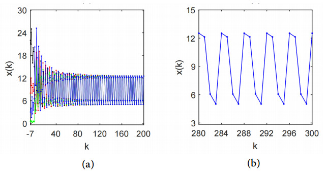
In this paper, we investigate the multiplicity of positive periodic solutions of a discrete blood cell production model with impulse effects. This model is described by periodic coefficients and time delays, as well as nonlinear feedback with exponential terms. By employing the Krasnosel'skii fixed point theorem, we establish a sufficient condition for the existence of at least two positive periodic solutions. To this end, we construct solution transformation between an impulsive delay difference equation and the corresponding nonimpulsive delay difference equation. Aditionally, a solution representation of the positive periodic solution of the blood cell production model is presented. Moreover, a numerical example and its simulations are given to illustrate the main result.
Citation: Yan Yan. Multiplicity of positive periodic solutions for a discrete impulsive blood cell production model[J]. AIMS Mathematics, 2023, 8(11): 26515-26531. doi: 10.3934/math.20231354
In this paper, we investigate the multiplicity of positive periodic solutions of a discrete blood cell production model with impulse effects. This model is described by periodic coefficients and time delays, as well as nonlinear feedback with exponential terms. By employing the Krasnosel'skii fixed point theorem, we establish a sufficient condition for the existence of at least two positive periodic solutions. To this end, we construct solution transformation between an impulsive delay difference equation and the corresponding nonimpulsive delay difference equation. Aditionally, a solution representation of the positive periodic solution of the blood cell production model is presented. Moreover, a numerical example and its simulations are given to illustrate the main result.

| [1] | K. Fiedler, C. Brunner, Mechanisms controlling hematopoiesis, In: Hematology–Science and practice, 2012. |
| [2] |
C. J. Zhuge, M. C. Mackey, J. Z. Lei, Origins of oscillation patterns in cyclical thrombocytopenia, J. Theor. Biol., 462 (2019), 432–445. https://doi.org/10.1016/j.jtbi.2018.11.024 doi: 10.1016/j.jtbi.2018.11.024

|
| [3] |
D. R. Boggs, Homeostatic regulatory mechanisms of hematopoiesis, Annu. Rev. Physiol., 28 (1966), 39–56. https://doi.org/10.1146/annurev.ph.28.030166.000351 doi: 10.1146/annurev.ph.28.030166.000351
|
| [4] |
C. Foley, M. C. Mackey, Dynamic hematological disease: A review, J. Math. Biol., 58 (2009), 285–322. https://doi.org/10.1007/s00285-008-0165-3 doi: 10.1007/s00285-008-0165-3
|
| [5] |
M. C. Mackey, J. G. Milton, Dynamical disease, Ann. New York Acad. Sci., 504 (1987), 16–32. https://doi.org/10.1111/j.1749-6632.1987.tb48723.x doi: 10.1111/j.1749-6632.1987.tb48723.x
|
| [6] | L. Glass, M. C. Mackey, From clocks to chaos: The rhythms of life, Princeton University Press, 1988. |
| [7] | S. Wiggins, Introduction to applied nonlinear dynamical systems and chaos, New York: Springer, 1990. |
| [8] | B. Balachandran, T. Kalm-Nagy, D. E. Gilsinn, Delay differential equations, New York: Springer, 2009. https://doi.org/10.1007/978-0-387-85595-0 |
| [9] |
J. Lelkes, T. Kalmar-Nagy, Bifurcation analysis of a forced delay equation for machine tool vibrations, Nonlinear Dyn., 98 (2019), 2961–2974. https://doi.org/10.1007/s11071-019-04984-w doi: 10.1007/s11071-019-04984-w
|
| [10] |
Y. L. Song, Y. H. Peng, T. H. Zhang, The spatially inhomogeneous Hopf bifurcation induced by memory delay in a memory-based diffusion system, J. Differ. Equ., 300 (2021), 597–624. https://doi.org/10.1016/j.jde.2021.08.010 doi: 10.1016/j.jde.2021.08.010
|
| [11] |
M. C. Mackey, L. Glass, Oscillation and chaos in physiological control systems, Science, 197 (1977), 287–289. https://doi.org/10.1126/science.267326 doi: 10.1126/science.267326
|
| [12] | A. Lasota, Ergodic problems in biology, Asterisque, 50 (1977), 239–250. |
| [13] |
L. Berezansky, E. Braverman, L. Idels, Mackey-Glass model of hematopoiesis with monotone feedback revisited, Appl. Math. Comput., 219 (2013), 4892–4907. https://doi.org/10.1016/j.amc.2012.10.052 doi: 10.1016/j.amc.2012.10.052
|
| [14] |
L. Berezansky, E. Braverman, L. Idels, Mackey-Glass model of hematopoiesis with non-monotone feedback: Stability, oscillation and control, Appl. Math. Comput., 219 (2013), 6268–6283. https://doi.org/10.1016/j.amc.2012.12.043 doi: 10.1016/j.amc.2012.12.043
|
| [15] |
G. R. Liu, J. R. Yan, F. Q. Zhang, Existence and global attractivity of unique positive periodic solution for a model of hematopoiesis, J. Math. Anal. Appl., 334 (2007), 157–171. https://doi.org/10.1016/j.jmaa.2006.12.015 doi: 10.1016/j.jmaa.2006.12.015
|
| [16] |
X. M. Wu, J. W. Li, H. Q. Zhou, A necessary and sufficient condition for the existence of positive periodic solutions of a model of hematopoiesis, Comput. Math. Appl., 54 (2007), 840–849. https://doi.org/10.1016/j.camwa.2007.03.004 doi: 10.1016/j.camwa.2007.03.004
|
| [17] |
Z. J. Yao, Existence and global attractivity of the unique positive periodic solution for discrete hematopoiesis model, Topol. Methods Nonlinear Anal., 45 (2015), 423–437. https://doi.org/10.12775/TMNA.2015.021 doi: 10.12775/TMNA.2015.021
|
| [18] |
Y. Yan, J. Sugie, Existence regions of positive periodic solutions for a discrete hematopoiesis model with unimodal production functions, Appl. Math. Model., 68 (2019), 152–168. https://doi.org/10.1016/j.apm.2018.11.003 doi: 10.1016/j.apm.2018.11.003
|
| [19] |
A. Halik, Dynamics in a two species Lotka-Volterra cooperative system with the Crowley-Martin functional response, J. Nonlinear Funct. Anal., 2021 (2021), 1–8. https://doi.org/10.23952/jnfa.2021.36 doi: 10.23952/jnfa.2021.36
|
| [20] |
W. H. Jiang, The existence of multiple positive periodic solutions for functional differential equations, Appl. Math. Comput., 208 (2009), 165–171. https://doi.org/10.1016/j.amc.2008.11.021 doi: 10.1016/j.amc.2008.11.021
|
| [21] |
M. Kamenskii, G. Petrosyan, C. F. Wen, An existence result for a periodic boundary value problem of fractional semilinear differential equations in a Banach space, J. Nonlinear Var. Anal., 5 (2021), 155–177. https://doi.org/10.23952/jnva.5.2021.1.10 doi: 10.23952/jnva.5.2021.1.10
|
| [22] |
J. W. Li, C. X. Du, Existence of positive periodic solutions for a generalized Nicholson's blowflies model, J. Comput. Appl. Math., 221 (2008), 226–233. https://doi.org/10.1016/j.cam.2007.10.049 doi: 10.1016/j.cam.2007.10.049
|
| [23] |
T. Faria, J. J. Oliveira, Global asymptotic stability for a periodic delay hematopoiesis model with impulses, Appl. Math. Model., 79 (2020), 843–864. https://doi.org/10.1016/j.apm.2019.10.063 doi: 10.1016/j.apm.2019.10.063
|
| [24] |
C. J. Gregory, E. A. McCulloch, J. K. Till, Erythropoietic progenitors capable of colony formation in culture: State of differentiation, J. Cell. Physiol., 81 (1973), 411–420. https://doi.org/10.1002/jcp.1040810313 doi: 10.1002/jcp.1040810313
|
| [25] |
J. C. Panetta, A mathematical model of periodically pulsed chemotherapy: Tumor recurrence and metastasis in a competitive environment, Bull. Math. Biol., 58 (1996), 425–447. https://doi.org/10.1007/BF02460591 doi: 10.1007/BF02460591
|
| [26] |
X. Z. Fu, Q. X. Zhu, Stability of nonlinear impulsive stochastic systems with Markovian switching under generalized average dwell time condition, Sci. China Inform. Sci., 61 (2018), 1–15. https://doi.org/10.1007/s11432-018-9496-6 doi: 10.1007/s11432-018-9496-6
|
| [27] |
W. Hu, Q. X. Zhu, Stability criteria for impulsive stochastic functional differential systems with distributed-delay dependent impulsive effects, IEEE Trans. Syst. Man Cybern. Syst., 51 (2021), 2027–2032. https://doi.org/10.1109/TSMC.2019.2905007 doi: 10.1109/TSMC.2019.2905007
|
| [28] |
W. Hu, Q. X. Zhu, H. R. Karimi, Some improved Razumikhin stability criteria for impulsive stochastic delay differential systems, IEEE Trans. Automat. Control, 64 (2019), 5207–5213. https://doi.org/10.1109/TAC.2019.2911182 doi: 10.1109/TAC.2019.2911182
|
| [29] |
G. D. Li, Y. Zhang, Y. J. Guan, W. J. Li, Stability analysis of multi-point boundary conditions for fractional differential equation with non-instantaneous integral impulse, Math. Biosci. Eng., 20 (2023), 7020–7041. https://doi.org/10.3934/mbe.2023303 doi: 10.3934/mbe.2023303
|
| [30] |
R. F. Rao, Z. Lin, X. Q. Ai, J. R. Wu, Synchronization of epidemic systems with Neumann boundary value under delayed impulse, Mathematics, 10 (2022), 1–10. https://doi.org/10.3390/math10122064 doi: 10.3390/math10122064
|
| [31] |
Y. Tang, L. Zhou, J. H. Tang, Y. Rao, H. G. Fan, J. H. Zhu, Hybrid impulsive pinning control for mean square synchronization of uncertain multi-link complex networks with stochastic characteristics and hybrid delays, Mathematics, 11 (2023), 1–18. https://doi.org/10.3390/math11071697 doi: 10.3390/math11071697
|
| [32] |
M. L. Xia, L. N. Liu, J. Y. Fang, Y. C. Zhang, Stability analysis for a class of stochastic differential equations with impulses, Mathematics, 11 (2023), 1–10. https://doi.org/10.3390/math11061541 doi: 10.3390/math11061541
|
| [33] |
Y. M. Xue, J. K. Han, Z. Q. Tu, X. Y. Chen, Stability analysis and design of cooperative control for linear delta operator system, AIMS Math., 8 (2023), 12671–12693. https://doi.org/10.3934/math.2023637 doi: 10.3934/math.2023637
|
| [34] |
Y. X. Zhao, L. S. Wang, Practical exponential stability of impulsive stochastic food chain system with time-varying delays, Mathematics, 11 (2023), 1–12. https://doi.org/10.3390/math11010147 doi: 10.3390/math11010147
|
| [35] |
T. Faria, R. Figueroa, Positive periodic solutions for systems of impulsive delay differential equations, Discrete Contin. Dyn. Syst. B, 28 (2023), 170–196. https://doi.org/10.3934/dcdsb.2022070 doi: 10.3934/dcdsb.2022070
|
| [36] |
Z. G. Luo, Multiple positive periodic solutions for two kinds of higher-dimension impulsive differential equations with multiple delays and two parameters, J. Math., 2014 (2014), 1–13. https://doi.org/10.1155/2014/214093 doi: 10.1155/2014/214093
|
| [37] |
Y. X. Tan, M. M. Zhang, Global exponential stability of periodic solutions in a nonsmooth model of hematopoiesis with time-varying delays, Math. Methods Appl. Sci., 40 (2017), 5986–5995. https://doi.org/10.1002/mma.4448 doi: 10.1002/mma.4448
|
| [38] |
J. R. Yan, Existence and global attractivity of positive periodic solution for an impulsive Lasota-Wazewska model, J. Math. Anal. Appl., 279 (2003), 111–120. https://doi.org/10.1016/S0022-247X(02)00613-3 doi: 10.1016/S0022-247X(02)00613-3
|
| [39] | M. A. Krasnosel'skii, Positive solutions of operator equations, Groningen: Noordhoff, 1964. |
Figures(1)

Yan Yan. Multiplicity of positive periodic solutions for a discrete impulsive blood cell production model[J]. AIMS Mathematics, 2023, 8(11): 26515-26531. doi: 10.3934/math.20231354


 DownLoad: