Aczel-Alsina t-norm and t-conorm are great substitutes for sum and product and recently various scholars developed notions based on the Aczel-Alsina t-norm and t-conorm. The theory of bipolar complex fuzzy set that deals with ambiguous and complex data that contains positive and negative aspects along with a second dimension. So, based on Aczel-Alsina operational laws and the dominant structure of the bipolar complex fuzzy set, we develop the notion of bipolar complex fuzzy Aczel-Alsina weighted geometric, bipolar complex fuzzy Aczel Alsina ordered weighted geometric and bipolar complex fuzzy Aczel Alsina hybrid geometric operators. Moreover, multi-attribute border approximation area comparison technique is a valuable technique that can cover many decision-making situations and have dominant results. So, based on bipolar complex fuzzy Aczel-Alsina aggregation operators, we demonstrate the notion of a multi-attribute border approximation area comparison approach for coping with bipolar complex fuzzy information. After that, we take a numerical example by taking artificial data for various types of operating systems and determining the finest operating system for a computer. In the end, we compare the deduced multi-attribute border approximation area comparison approach and deduced aggregation operators with numerous prevailing works.
Citation: Tahir Mahmood, Azam, Ubaid ur Rehman, Jabbar Ahmmad. Prioritization and selection of operating system by employing geometric aggregation operators based on Aczel-Alsina t-norm and t-conorm in the environment of bipolar complex fuzzy set[J]. AIMS Mathematics, 2023, 8(10): 25220-25248. doi: 10.3934/math.20231286
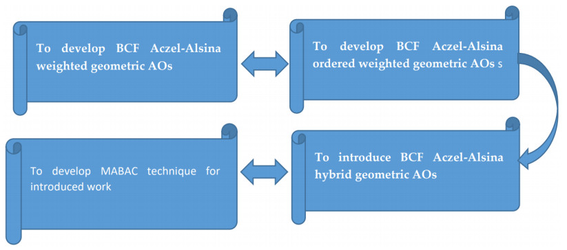
Aczel-Alsina t-norm and t-conorm are great substitutes for sum and product and recently various scholars developed notions based on the Aczel-Alsina t-norm and t-conorm. The theory of bipolar complex fuzzy set that deals with ambiguous and complex data that contains positive and negative aspects along with a second dimension. So, based on Aczel-Alsina operational laws and the dominant structure of the bipolar complex fuzzy set, we develop the notion of bipolar complex fuzzy Aczel-Alsina weighted geometric, bipolar complex fuzzy Aczel Alsina ordered weighted geometric and bipolar complex fuzzy Aczel Alsina hybrid geometric operators. Moreover, multi-attribute border approximation area comparison technique is a valuable technique that can cover many decision-making situations and have dominant results. So, based on bipolar complex fuzzy Aczel-Alsina aggregation operators, we demonstrate the notion of a multi-attribute border approximation area comparison approach for coping with bipolar complex fuzzy information. After that, we take a numerical example by taking artificial data for various types of operating systems and determining the finest operating system for a computer. In the end, we compare the deduced multi-attribute border approximation area comparison approach and deduced aggregation operators with numerous prevailing works.

| [1] | P. B. Hansen, Operating system principles, United States: Prentice-Hall, Inc., 1973. Available from: https://dl.acm.org/doi/abs/10.5555/540365. |
| [2] | A. Silberschatz, P. B. Galvin, G. Gagne, Applied operating system concepts, United States: John Wiley and Sons, Inc., 1999. Available from: https://dl.acm.org/doi/abs/10.5555/330796. |
| [3] | D. Comer, Operating system design, New York: CRC Press, 2011. |
| [4] | G. Klein, Operating system verification—an overview, Springer, 34 (2009), 27–69. https://doi.org/10.1007/s12046-009-0002-4 |
| [5] | C. W. Mercer, Operating system support for multimedia applications, In: Proceedings of the second ACM international conference on Multimedia, 1994,492–493. https://doi.org/10.1145/192593.197424 |
| [6] | S. T. King, G. W. Dunlap, P. M. Chen, Operating system support for virtual machines, In: USENIX Annual Technical Conference, General Track, 2003, 71–84. |
| [7] | I. M. Leslie, D. McAuley, R. Black, T. Roscoe, P. Barham, D. Evers, et al., The design and implementation of an operating system to support distributed multimedia applications, IEEE J. Sel. Area. Comm., 14 (1996), 1280–1297. https://doi.org/10.1109/49.536480 |
| [8] | R. Singh, An overview of the android operating system and its security, Int. J. Eng. Res. Appl., 4 (2014), 519–521. |
| [9] | L. A. Zadeh, Fuzzy sets, Inf. Control, 8 (1965), 338–353. https://doi.org/10.1016/S0019-9958(65)90241-X |
| [10] | H. J. Zimmermann, Fuzzy set theory—and its applications, 4 Eds, Springer Sci., 2011. |
| [11] |
M. Riaz, M. R. Hashmi, D. Pamucar, Y. M. Ch, Spherical linear Diophantine fuzzy sets with modeling uncertainties in MCDM, Comput. Model. Eng. Sci., 126 (2021), 1125–1164. https://doi.org/10.32604/cmes.2021.013699 doi: 10.32604/cmes.2021.013699

|
| [12] |
S. Ayub, M. Shabir, M. Riaz, W. Mahmood, D. Bozanic, D. Marinkovic, Linear Diophantine fuzzy rough sets: A new rough set approach with decision making, Symmetry, 14 (2022), 525. https://doi.org/10.3390/sym14030525 doi: 10.3390/sym14030525
|
| [13] |
M. Riaz, M. R. Hashmi, Linear Diophantine fuzzy set and its applications towards multi-attribute decision-making problems, J. Intell. Fuzzy Syst., 37 (2019), 5417–5439. https://doi.org/10.3233/JIFS-190550 doi: 10.3233/JIFS-190550
|
| [14] |
E. Tolga, M. L. Demircan, C. Kahraman, Operating system selection using fuzzy replacement analysis and analytic hierarchy process, Int. J. Prod. Econ., 97 (2005), 89–117. https://doi.org/10.1016/j.ijpe.2004.07.001 doi: 10.1016/j.ijpe.2004.07.001
|
| [15] |
S. Ballı, S. Korukoğlu, Operating system selection using fuzzy AHP and TOPSIS methods, Math. Comput. Appl., 14 (2009), 119–130. https://doi.org/10.3390/mca14020119 doi: 10.3390/mca14020119
|
| [16] |
A. Kandel, Y. Q. Zhang, M. Henne, On the use of fuzzy logic technology in operating systems, Fuzzy Set. Syst., 99 (1998), 241–251. https://doi.org/10.1016/S0165-0114(96)00392-2 doi: 10.1016/S0165-0114(96)00392-2
|
| [17] |
A. Mardani, M. Nilashi, E. K. Zavadskas, S. R. Awang, H. Zare, N. M. Jamal, Decision making methods based on fuzzy aggregation operators: Three decades review from 1986 to 2017, Int. J. Inf. Technol. Decisi. Mak., 17 (2018), 391–466. https://doi.org/10.1142/S021962201830001X doi: 10.1142/S021962201830001X
|
| [18] | W. R. Zhang, Bipolar fuzzy sets and relations: A computational framework for cognitive modeling and multiagent decision analysis, In: NAFIPS/IFIS/NASA'94, Proceedings of the First International Joint Conference of The North American Fuzzy Information Processing Society Biannual Conference, The Industrial Fuzzy Control and Intellige, 1994,305–309. https://doi.org/10.1109/IJCF.1994.375115 |
| [19] |
G. Wei, F. E. Alsaadi, T. Hayat, A. Alsaedi, Bipolar fuzzy Hamacher aggregation operators in multiple attribute decision making, Int. J. Fuzzy Syst., 20 (2018), 1–12. https://doi.org/10.1007/s40815-017-0338-6 doi: 10.1007/s40815-017-0338-6
|
| [20] |
C. Jana, M. Pal, J. Q. Wang, Bipolar fuzzy Dombi aggregation operators and its application in multiple-attribute decision-making process, J. Amb. Intel. Hum. Comp., 10 (2019), 3533–3549. https://doi.org/10.1007/s12652-018-1076-9 doi: 10.1007/s12652-018-1076-9
|
| [21] | M. Akram, Bipolar fuzzy graphs, Inf. Sci., 181 (2011), 5548–5564. https://doi.org/10.1016/j.ins.2011.07.037 |
| [22] |
M. Akram, Bipolar fuzzy graphs with applications, Knowl.-Based Syst., 39 (2013), 1–8. https://doi.org/10.1016/j.knosys.2012.08.022 doi: 10.1016/j.knosys.2012.08.022
|
| [23] | S. Samanta, M. Pal, Irregular bipolar fuzzy graphs, arXiv preprint, 2012. https://doi.org/10.48550/arXiv.1209.1682 |
| [24] |
H. Rashmanlou, S. Samanta, M. Pal, R. A. Borzooei, Product of bipolar fuzzy graphs and their degree, Int. J. Gen. Syst., 45 (2016), 1–14. https://doi.org/10.1080/03081079.2015.1072521 doi: 10.1080/03081079.2015.1072521
|
| [25] |
M. A. Alghamdi, N. O. Alshehri, M. Akram, Multi-criteria decision-making methods in bipolar fuzzy environment, Int. J. Fuzzy Syst., 20 (2018), 2057–2064. https://doi.org/10.1007/s40815-018-0499-y doi: 10.1007/s40815-018-0499-y
|
| [26] |
M. Akram, M. Ali, T. Allahviranloo, A method for solving bipolar fuzzy complex linear systems with real and complex coefficients, Soft Comput., 26 (2022), 2157–2178. https://doi.org/10.1007/s00500-021-06672-7 doi: 10.1007/s00500-021-06672-7
|
| [27] |
M. Akram, U. Amjad, B. Davvaz, Decision-making analysis based on bipolar fuzzy N-soft information, Comput. Appl. Math., 40 (2021), 182. https://doi.org/10.1007/s40314-021-01570-y doi: 10.1007/s40314-021-01570-y
|
| [28] | M. Akram, A. N. Al-Kenani, Multi-criteria group decision-making for selection of green suppliers under bipolar fuzzy PROMETHEE process, Symmetry, 12 (2020), 77. https://doi.org/10.3390/sym12010077 |
| [29] |
M. Akram, Shumaiza, M. Arshad, Bipolar fuzzy TOPSIS and bipolar fuzzy ELECTRE-I methods to diagnosis, Comput. Appl. Math., 39 (2020), 1–21. https://doi.org/10.1007/s40314-019-0980-8 doi: 10.1007/s40314-019-0980-8
|
| [30] |
M. Akram, A. N. Al-Kenani, J. C. R. Alcantud, Group decision-making based on the VIKOR method with trapezoidal bipolar fuzzy information, Symmetry, 11 (2019), 1313. https://doi.org/10.3390/sym11101313 doi: 10.3390/sym11101313
|
| [31] |
M. Akram, M. Arshad, A novel trapezoidal bipolar fuzzy TOPSIS method for group decision-making, Group Decis. Negot., 28 (2019), 565–584. https://doi.org/10.1007/s10726-018-9606-6 doi: 10.1007/s10726-018-9606-6
|
| [32] | M. Akram, M. Ali, T. Allahviranloo, Solution of the complex bipolar fuzzy linear system, In: Progress in Intelligent Decision Science, Springer, Cham, 1301 (2021), 899–927. https://doi.org/10.1007/978-3-030-66501-2-73 |
| [33] |
C. Jana, M. Pal, J. Q. Wang, Bipolar fuzzy Dombi prioritized aggregation operators in multiple attribute decision making, Soft Comput., 24 (2020), 3631–3646. https://doi.org/10.1007/s00500-019-04130-z doi: 10.1007/s00500-019-04130-z
|
| [34] |
M. Riaz, S. T. Tehrim, Multi-attribute group decision making based on cubic bipolar fuzzy information using averaging aggregation operators, J. Intell. Fuzzy Syst., 37 (2019), 2473–2494. https://doi.org/10.3233/JIFS-182751 doi: 10.3233/JIFS-182751
|
| [35] | D. Ramot, R. Milo, M. Friedman, A. Kandel, Complex fuzzy sets, IEEE T. Fuzzy Syst. 10 (2002), 171–186. https://doi.org/10.1109/91.995119 |
| [36] |
D. E. Tamir, L. Jin, A. Kandel, A new interpretation of complex membership grade, Int. J. Intell. Syst., 26 (2011), 285–312. https://doi.org/10.1002/int.20454 doi: 10.1002/int.20454
|
| [37] | D. E. Tamir, N. D. Rishe, A. Kandel, Complex fuzzy sets and complex fuzzy logic an overview of theory and applications, In: Fifty years of fuzzy logic and its applications, Springer, Cham, 326 (2015), 661–681. https://doi.org/10.1007/978-3-319-19683-1-31 |
| [38] | L. Bi, S. Dai, B. Hu, Complex fuzzy geometric aggregation operators, Symmetry, 10 (2018), 251. https://doi.org/10.3390/sym10070251 |
| [39] |
L. Bi, S. Dai, B. Hu, S. Li, Complex fuzzy arithmetic aggregation operators, J. Intell. Fuzzy Syst., 36 (2019), 2765–2771. https://doi.org/10.3233/JIFS-18568 doi: 10.3233/JIFS-18568
|
| [40] | T. Mahmood, U. Ur Rehman, A novel approach towards bipolar complex fuzzy sets and their applications in generalized similarity measures, Int. J. Intell. Syst., 37 (2022), 535–567. https://doi.org/10.1002/int.22639 |
| [41] | T. Mahmood, U. Ur Rehman, A method to multi-attribute decision making technique based on Dombi aggregation operators under bipolar complex fuzzy information, Comput. Appl. Math., 41 (2022), 1–23. https://doi.org/10.1007/s40314-021-01735-9 |
| [42] |
T. Mahmood, U. Ur Rehman, Z. Ali, Analysis and application of Aczel-Alsina aggregation operators based on bipolar complex fuzzy information in multiple attribute decision making, Inf. Sci., 619 (2023), 817–833. https://doi.org/10.1016/j.ins.2022.11.067 doi: 10.1016/j.ins.2022.11.067
|
| [43] | D. Pamučar, G. Ćirović, The selection of transport and handling resources in logistics centers using Multi-Attributive Border Approximation Area Comparison (MABAC), Expert Syst. Appl., 42 (2015), 3016–3028. https://doi.org/10.1016/j.eswa.2014.11.057 |
| [44] |
R. Verma, Fuzzy MABAC method based on new exponential fuzzy information measures, Soft Comput., 25 (2021), 9575–9589. https://doi.org/10.1007/s00500-021-05739-9 doi: 10.1007/s00500-021-05739-9
|
| [45] |
M. Zhao, G. Wei, X. Chen, Y. Wei, Intuitionistic fuzzy MABAC method based on cumulative prospect theory for multiple attribute group decision making, Int. J. Intel. Syst., 36 (2021), 6337–6359. https://doi.org/10.1002/int.22552 doi: 10.1002/int.22552
|
| [46] |
Z. Jiang, G. Wei, Y. Guo, Picture fuzzy MABAC method based on prospect theory for multiple attribute group decision making and its application to suppliers' selection, J. Intel. Fuzzy. Syst., 42 (2022), 3405–3415. https://doi.org/10.3233/JIFS-211359 doi: 10.3233/JIFS-211359
|
| [47] |
C. Jana, Multiple attribute group decision-making method based on extended bipolar fuzzy MABAC approach, Comput. Appl. Math., 40 (2021), 1–17. https://doi.org/10.1007/s40314-021-01606-3 doi: 10.1007/s40314-021-01606-3
|
| [48] |
R. Zhang, Z. Xu, X. Gou, ELECTRE Ⅱ method based on the cosine similarity to evaluate the performance of financial logistics enterprises under a double hierarchy hesitant fuzzy linguistic environment, Fuzzy Optim. Decis. Ma., 22 (2023), 23–49. https://doi.org/10.1007/s10700-022-09382-3 doi: 10.1007/s10700-022-09382-3
|
| [49] |
X. Gou, Z. Xu, H. Liao, F. Herrera, Probabilistic double hierarchy linguistic term set and its use in designing an improved VIKOR method: The application in smart healthcare, J. Oper. Res. Soc., 72 (2021), 2611–2630. https://doi.org/10.1080/01605682.2020.1806741 doi: 10.1080/01605682.2020.1806741
|
| [50] |
X. Gou, Z. Xu, H. Liao, Hesitant fuzzy linguistic entropy and cross-entropy measures and alternative queuing method for multiple criteria decision making, Inf. Sci., 388 (2017), 225–246. https://doi.org/10.1016/j.ins.2017.01.033 doi: 10.1016/j.ins.2017.01.033
|
| [51] | X. Gou, X. Xu, F. Deng, W. Zhou, E. Herrera-Viedma, Correction: Medical health resources allocation evaluation in public health emergencies by an improved ORESTE method with linguistic preference orderings, Fuzzy Optim. Decis. Ma., 2023. https://doi.org/10.1007/s10700-023-09409-3 |
| [52] |
J. Aczel, C. Alsina, Characterizations of some classes of quasilinear functions with applications to triangular norms and synthesizing judgments, Aequationes Math., 25 (1982), 313–315. https://doi.org/10.1007/BF02189626 doi: 10.1007/BF02189626
|
| [53] |
T. Senapati, G. Chen, R. R. Yager, Aczel-Alsina aggregation operators and their application to intuitionistic fuzzy multiple attribute decision making, Intel. J. Fuzzy. Syst., 37 (2022), 1529–1551. https://doi.org/10.1002/int.22684 doi: 10.1002/int.22684
|
| [54] |
T. Senapati, G. Chen, R. Mesiar, R. R. Yager, Novel Aczel-Alsina operations-based interval-valued intuitionistic fuzzy aggregation operators and their applications in multiple attribute decision-making process, Intel. J. Fuzzy Syst., 37 (2022), 5059–5081. https://doi.org/10.1002/int.22751 doi: 10.1002/int.22751
|
| [55] |
T. Senapati, Approaches to multi-attribute decision-making based on picture fuzzy Aczel-Alsina average aggregation operators, Comput. Appl. Math., 41 (2022), 40. https://doi.org/10.1007/s40314-021-01742-w doi: 10.1007/s40314-021-01742-w
|
| [56] | A. Hussain, K. Ullah, M. S. Yang, D. Pamucar, Aczel-Alsina aggregation operators on T-spherical fuzzy (TSF) information with application to TSF multi-attribute decision making, IEEE Access, 10 (2022), 26011–26023. |
| [57] | W. Ali, T. Shaheen, I. U. Haq, H. Toor, F. Akram, H. Garg, et al., Aczel-Alsina-based aggregation operators for intuitionistic hesitant fuzzy set environment and their application to multiple attribute decision-making process, AIMS Math., 8 (2023), 18021–18039. https://doi.org/10.3934/math.2023916 |
| [58] |
M. Palanikumar, N. Kausar, H. Garg, S. F. Ahmed, C. Samaniego, Robot sensors process based on generalized Fermatean normal different aggregation operator's framework, AIMS Math., 8 (2023), 16252–16277. https://doi.org/10.3934/math.2023832 doi: 10.3934/math.2023832
|
| [59] |
J. Ahmmad, T. Mahmood, R. Chinram, A. Iampan, Some average aggregation operators based on spherical fuzzy soft sets and their applications in multi-criteria decision making, AIMS Math., 6 (2021), 7798–7833. https://doi.org/10.3934/math.2021454 doi: 10.3934/math.2021454
|
| [60] |
J. Zhan, J. Deng, Z. Xu, L. Martínez, A three-way decision methodology with regret theory via triangular fuzzy numbers in incomplete multi-scale decision information systems, IEEE T. Fuzzy Syst., 31 (2023), 2773–2787. https://doi.org/10.1109/TFUZZ.2023.3237646 doi: 10.1109/TFUZZ.2023.3237646
|
| [61] |
J. Zhu, X. Ma, G. Kou, E. Herrera-Viedma, J. Zhan, A three-way consensus model with regret theory under the framework of probabilistic linguistic term sets, Inform. Fusion, 95 (2023), 250–274. https://doi.org/10.1016/j.inffus.2023.02.029 doi: 10.1016/j.inffus.2023.02.029
|


Figures(4) / Tables(9)

Tahir Mahmood, Azam, Ubaid ur Rehman, Jabbar Ahmmad. Prioritization and selection of operating system by employing geometric aggregation operators based on Aczel-Alsina t-norm and t-conorm in the environment of bipolar complex fuzzy set[J]. AIMS Mathematics, 2023, 8(10): 25220-25248. doi: 10.3934/math.20231286


 DownLoad: