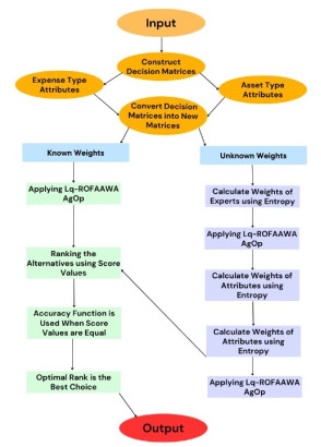
In this article, we presented two novel approaches for group decision-making (GDM) that were derived from the initiated linguistic $ q $-rung orthopair fuzzy Aczel-Alsina weighted arithmetic (L$ q $-ROFAAWA) aggregation operator (AgOp) using linguistic $ q $-rung orthopair fuzzy numbers (L$ q $-ROFNs). To introduce these GDM techniques, we first defined new operational laws for L$ q $-ROFNs based on Aczel-Alsina $ t $-norm and $ t $-conorm. The developed scalar multiplication and addition operations of L$ q $-ROFNs addressed the limitations of operations when $ q = 1 $. The first proposed GDM methodology assumed that both experts' weights and attribute weights were fully known, while the second technique assumed that both sets of weights were entirely unknown. We also discussed properties of L$ q $-ROFNs under the L$ q $-ROFAAWA operators, such as idempotency, boundedness, and monotonicity. Furthermore, we solved problems related to environmental and economic issues, such as ranking countries by air pollution, selecting the best company for bank investments, and choosing the best electric vehicle design. Finally, we validated the proposed GDM approaches using three validity tests and performed a sensitivity analysis to compare them with preexisting models.
Citation: Ghous Ali, Kholood Alsager, Asad Ali. Novel linguistic $ q $-rung orthopair fuzzy Aczel-Alsina aggregation operators for group decision-making with applications[J]. AIMS Mathematics, 2024, 9(11): 32328-32365. doi: 10.3934/math.20241551
In this article, we presented two novel approaches for group decision-making (GDM) that were derived from the initiated linguistic $ q $-rung orthopair fuzzy Aczel-Alsina weighted arithmetic (L$ q $-ROFAAWA) aggregation operator (AgOp) using linguistic $ q $-rung orthopair fuzzy numbers (L$ q $-ROFNs). To introduce these GDM techniques, we first defined new operational laws for L$ q $-ROFNs based on Aczel-Alsina $ t $-norm and $ t $-conorm. The developed scalar multiplication and addition operations of L$ q $-ROFNs addressed the limitations of operations when $ q = 1 $. The first proposed GDM methodology assumed that both experts' weights and attribute weights were fully known, while the second technique assumed that both sets of weights were entirely unknown. We also discussed properties of L$ q $-ROFNs under the L$ q $-ROFAAWA operators, such as idempotency, boundedness, and monotonicity. Furthermore, we solved problems related to environmental and economic issues, such as ranking countries by air pollution, selecting the best company for bank investments, and choosing the best electric vehicle design. Finally, we validated the proposed GDM approaches using three validity tests and performed a sensitivity analysis to compare them with preexisting models.

| [1] |
L. A. Zadeh, Fuzzy sets, Information and Control, 8 (1965), 338–353. https://doi.org/10.1016/S0019-9958(65)90241-X doi: 10.1016/S0019-9958(65)90241-X

|
| [2] |
R. E. Bellman, L. A. Zadeh, Decision-making in a fuzzy environment, Manage. Sci., 17 (1970), 141–164. https://doi.org/10.1287/mnsc.17.4.B141 doi: 10.1287/mnsc.17.4.B141
|
| [3] |
Z. Pawlak, Rough sets, International Journal of Computer and Information Sciences, 11 (1982), 341–356. https://doi.org/10.1007/BF01001956 doi: 10.1007/BF01001956
|
| [4] |
J. Q. Wang, X. H. Zhang, Q. Shen, Choquet-like integrals with rough attribute fuzzy measures for data-driven decision-making, IEEE T. Fuzzy Syst., 32 (2024), 2825–2836. https://doi.org/10.1109/TFUZZ.2024.3363415 doi: 10.1109/TFUZZ.2024.3363415
|
| [5] |
J. Q. Wang, X. H. Zhang, Intuitionistic fuzzy granular matrix: novel calculation approaches for intuitionistic, fuzzy covering-based rough sets, Axioms, 13 (2024), 411. https://doi.org/10.3390/axioms13060411 doi: 10.3390/axioms13060411
|
| [6] |
K. T. Atanassov, Intuitionistic fuzzy sets, Fuzzy Set. Syst., 20 (1986), 87–96. https://doi.org/10.1016/S0165-0114(86)80034-3 doi: 10.1016/S0165-0114(86)80034-3
|
| [7] | R. R. Yager, Pythagorean fuzzy subsets, 2013 Joint IFSA World Congress and NAFIPS Annual Meeting (IFSA/NAFIPS), Edmonton, AB, Canada, 2013, 57–61. https://doi.org/10.1109/IFSA-NAFIPS.2013.6608375 |
| [8] |
R. R. Yager, Generalized orthopair fuzzy sets, IEEE T. Fuzzy Syst., 25 (2017), 1222–1230. https://doi.org/10.1109/TFUZZ.2016.2604005 doi: 10.1109/TFUZZ.2016.2604005
|
| [9] |
L. A. Zadeh, The concept of a linguistic variable and its application to approximate reasoning–I, Inform. Sciences, 8 (1975), 199–249. https://doi.org/10.1016/0020-0255(75)90036-5 doi: 10.1016/0020-0255(75)90036-5
|
| [10] |
Z. C. Chen, P. H. Liu, Z. Pei, An approach to multiple attribute group decision making based on linguistic intuitionistic fuzzy numbers, Int. J. Comput. Int. Sys., 8 (2015), 747–760. https://doi.org/10.1080/18756891.2015.1061394 doi: 10.1080/18756891.2015.1061394
|
| [11] |
M. Akram, S. Naz, T. Abbas, Complex $q$-rung orthopair fuzzy 2-tuple linguistic group decision-making framework with Muirhead mean operators, Artif. Intell. Rev., 56 (2023), 10227–10274. https://doi.org/10.1007/s10462-023-10408-4 doi: 10.1007/s10462-023-10408-4
|
| [12] |
M. Akram, N. Ramzan, A. Luqman, G. Santos-García, An integrated MULTIMOORA method with 2-tuple linguistic Fermatean fuzzy sets: Urban quality of life selection application, AIMS Mathematics, 8 (2023), 2798–2828. https://doi.org/10.3934/math.2023147 doi: 10.3934/math.2023147
|
| [13] |
M. R. Seikh, U. Mandal, Interval-valued Fermatean fuzzy Dombi aggregation operators and SWARA based PROMETHEE II method to bio-medical waste management, Expert Syst. Appl., 226 (2023), 120082. https://doi.org/10.1016/j.eswa.2023.120082 doi: 10.1016/j.eswa.2023.120082
|
| [14] |
P. D. Liu, X. X. Liu, G. Y. Ma, Z. L. Liang, C. H. Wang, F. E. Alsaadi, A multi-attribute group decision-making method based on linguistic intuitionistic fuzzy numbers and Dempster-Shafer evidence theory, Int. J. Inf. Tech. Decis., 19 (2020), 499–524. https://doi.org/10.1142/S0219622020500042 doi: 10.1142/S0219622020500042
|
| [15] |
R. P. Yuan, J. Tang, F. Y. Meng, Linguistic intuitionistic fuzzy group decision making based on aggregation operators, Int. J. Fuzzy Syst., 21 (2019), 407–420. https://doi.org/10.1007/s40815-018-0582-4 doi: 10.1007/s40815-018-0582-4
|
| [16] |
X. J. Gou, X. R. Xu, F. M. Deng, W. Zhou, E. Herrera-Viedma, Medical health resources allocation evaluation in public health emergencies by an improved ORESTE method with linguistic preference orderings, Fuzzy Optim. Decis. Making, 23 (2024), 1–27. https://doi.org/10.1007/s10700-023-09409-3 doi: 10.1007/s10700-023-09409-3
|
| [17] |
X. T. Cheng, K. Zhang, T. Wu, Z. S. Xu, X. J. Gou, An opinions-updating model for large-scale group decision-making driven by autonomous learning, Inform. Sciences, 662 (2024), 120238. https://doi.org/10.1016/j.ins.2024.120238 doi: 10.1016/j.ins.2024.120238
|
| [18] |
M. R. Seikh, U. Mandal, $q$-Rung orthopair fuzzy Archimedean aggregation operators: application in the site selection for software operating units, Symmetry, 15 (2023), 1680. https://doi.org/10.3390/sym15091680 doi: 10.3390/sym15091680
|
| [19] |
M. R. Seikh, U. Mandal, Q-Rung orthopair fuzzy Frank aggregation operators and its application in multiple attribute decision-making with unknown attribute weights, Granul. Comput., 7 (2022), 709–730. https://doi.org/10.1007/s41066-021-00290-2 doi: 10.1007/s41066-021-00290-2
|
| [20] | H. Garg, K. Kumar, Group decision making approach based on possibility degree measures and the linguistic intuitionistic fuzzy aggregation operators using Einstein norm operations, J. Mult.-Valued Log. S., 31 (2018), 175–209. |
| [21] |
H. Garg, K. Kumar, Some aggregation operators for linguistic intuitionistic fuzzy set and its application to group decision-making process using the set pair analysis, Arab. J. Sci. Eng., 43 (2018), 3213–3227. https://doi.org/10.1007/s13369-017-2986-0 doi: 10.1007/s13369-017-2986-0
|
| [22] |
H. Garg, T. Mahmood, U. U. Rehman, G. N. Nguyen, Multi-attribute decision-making approach based on Aczel-Alsina power aggregation operators under bipolar fuzzy information and its application to quantum computing, Alex. Eng. J., 82 (2023), 248–259. https://doi.org/10.1016/j.aej.2023.09.073 doi: 10.1016/j.aej.2023.09.073
|
| [23] |
K. Kumar, S. M. Chen, Group decision making based on improved linguistic interval-valued Atanassov intuitionistic fuzzy weighted averaging aggregation operator of linguistic interval-valued Atanassov intuitionistic fuzzy numbers, Inform. Sciences, 607 (2022), 884–900. https://doi.org/10.1016/j.ins.2022.05.082 doi: 10.1016/j.ins.2022.05.082
|
| [24] |
K. Kumar, S. M. Chen, Multiple attribute group decision making based on advanced linguistic intuitionistic fuzzy weighted averaging aggregation operator of linguistic intuitionistic fuzzy numbers, Inform. Sciences, 587 (2022), 813–824. https://doi.org/10.1016/j.ins.2021.11.014 doi: 10.1016/j.ins.2021.11.014
|
| [25] | Y. Liu, G. W. Wei, H. B. Liu, L. Xu, Group decision making for internet public opinion emergency based upon linguistic intuitionistic fuzzy information, Int. J. Mach. Learn. & Cyber., 13 (2022), 579–594. https://doi.org/10.1007/s13042-020-01262-9 |
| [26] |
X. J. Gou, Z. S. Xu, H. C. Liao, F. Herrera, Probabilistic double hierarchy linguistic term set and its use in designing an improved VIKOR method: The application in smart healthcare, J. Oper. Res. Soc., 72 (2021), 2611–2630. https://doi.org/10.1080/01605682.2020.1806741 doi: 10.1080/01605682.2020.1806741
|
| [27] |
J. Tang, F. Y. Meng, Linguistic intuitionistic fuzzy Hamacher aggregation operators and their application to group decision making, Granul. Comput., 4 (2019), 109–124. https://doi.org/10.1007/s41066-018-0089-2 doi: 10.1007/s41066-018-0089-2
|
| [28] |
K. Kumar, S. M. Chen, Group decision making based on linguistic intuitionistic fuzzy Yager weighted arithmetic aggregation operator of linguistic intuitionistic fuzzy numbers, Inform. Sciences, 647 (2023), 119228. https://doi.org/10.1016/j.ins.2023.119228 doi: 10.1016/j.ins.2023.119228
|
| [29] |
R. Verma, N. Agarwal, Multiple attribute group decision-making based on generalized aggregation operators under linguistic interval-valued Pythagorean fuzzy environment, Granul. Comput., 7 (2022), 591–632. https://doi.org/10.1007/s41066-021-00286-y doi: 10.1007/s41066-021-00286-y
|
| [30] |
A. Fahmi, S. Abdullah, F. Amin, Aggregation operators on cubic linguistic hesitant fuzzy numbers and their application in group decision-making, Granul. Comput., 6 (2021), 303–320. https://doi.org/10.1007/s41066-019-00188-0 doi: 10.1007/s41066-019-00188-0
|
| [31] |
K. Kumar, S. M. Chen, Multiattribute decision making based on q-rung orthopair fuzzy Yager prioritized weighted arithmetic aggregation operator of q-rung orthopair fuzzy numbers, Inform. Sciences, 657 (2024), 119984. https://doi.org/10.1016/j.ins.2023.119984 doi: 10.1016/j.ins.2023.119984
|
| [32] |
X. T. Cheng, Z. S. Xu, X. J. Gou, A large-scale group decision-making model considering risk attitudes and dynamically changing roles, Expert Syst. Appl., 245 (2024), 123017. https://doi.org/10.1016/j.eswa.2023.123017 doi: 10.1016/j.eswa.2023.123017
|
| [33] |
F. X. Jin, F. Wang, K. Zhao, H. T. Chen, J. L. G. Guirao, The method of judging satisfactory consistency of linguistic judgment matrix based on adjacency matrix and 3-loop matrix, AIMS Mathematics, 9 (2024), 18944–18967. https://doi.org/10.3934/math.2024922 doi: 10.3934/math.2024922
|
| [34] |
M. W. Lin, X. M. Li, L. F. Chen, Linguistic q‐rung orthopair fuzzy sets and their interactional partitioned Heronian mean aggregation operators, Int. J. Intell. Syst., 35 (2019), 217–249. https://doi.org/10.1002/int.22136 doi: 10.1002/int.22136
|
| [35] |
P. D. Liu, W. Q. Liu, Multiple-attribute group decision-making based on power Bonferroni operators of linguistic q-rung orthopair fuzzy numbers, Int. J. Intell. Syst., 34 (2018), 652–689. https://doi.org/10.1002/int.22071 doi: 10.1002/int.22071
|
| [36] |
P. D. Liu, W. Q. Liu, Multiple‐attribute group decision‐making method of linguistic $q$‐rung orthopair fuzzy power Muirhead mean operators based on entropy weight, Int. J. Intell. Syst., 34 (2019), 1755–1794. https://doi.org/10.1002/int.22114 doi: 10.1002/int.22114
|
| [37] |
M. J. Ranjan, B. P. Kumar, T. D. Bhavani, A. V. Padmavathi, V. Bakka, Probabilistic linguistic q-rung orthopair fuzzy Archimedean aggregation operators for group decision-making, Decision Making: Applications in Management and Engineering, 6 (2023), 639–667. https://doi.org/10.31181/dmame622023527 doi: 10.31181/dmame622023527
|
| [38] |
H. J. Wang, Y. Liu, Y. Rong, Group decision making approach based on linguistic q-rung orthopair fuzzy generalized shapley bi-direction Choquet-copula operators, Granul. Comput., 8 (2023), 1837–1856. https://doi.org/10.1007/s41066-023-00404-y doi: 10.1007/s41066-023-00404-y
|
| [39] |
G. Ali, M. Afzal, M. Asif, A. Shazad, Attribute reduction approaches under interval-valued q-rung orthopair fuzzy soft framework, Appl. Intell., 52 (2022), 8975–9000. https://doi.org/10.1007/s10489-021-02853-x doi: 10.1007/s10489-021-02853-x
|
| [40] |
N. Deb, A. Sarkar, A. Biswas, Linguistic q-rung orthopair fuzzy prioritized aggregation operators based on Hamacher t-norm and t-conorm and their applications to multicriteria group decision making, Arch. Control Sci., 32 (2022), 451–484. https://doi.org/10.24425/acs.2022.141720 doi: 10.24425/acs.2022.141720
|
| [41] | P. D. Liu, S. Naz, M. Akram, M. Muzammal, Group decision-making analysis based on linguistic $q$-rung orthopair fuzzy generalized point weighted aggregation operators, Int. J. Mach. Learn. & Cyber., 13 (2022), 883–906. https://doi.org/10.1007/s13042-021-01425-2 |
| [42] |
M. Akram, S. Naz, S. A. Edalatpanah, R. Mehreen, Group decision-making framework under linguistic $q$-rung orthopair fuzzy Einstein models, Soft Comput., 25 (2021), 10309–10334. https://doi.org/10.1007/s00500-021-05771-9 doi: 10.1007/s00500-021-05771-9
|
| [43] |
C. Jana, M. Dobrodolac, V. Simic, M. Pal, B. Sarkar, Ž. Stević, Evaluation of sustainable strategies for urban parcel delivery: Linguistic $q$-rung orthopair fuzzy Choquet integral approach, Eng. Appl. Artif. Intel., 126 (2023), 106811. https://doi.org/10.1016/j.engappai.2023.106811 doi: 10.1016/j.engappai.2023.106811
|
| [44] | S. Naz, M. Akram, A. Shafiq, K. Akhtar, Optimal airport selection utilizing power Muirhead mean based group decision model with 2-tuple linguistic q-rung orthopair fuzzy information, Int. J. Mach. Learn. & Cyber., 15 (2024), 303–340. https://doi.org/10.1007/s13042-023-01911-9 |
| [45] |
J. Aczél, C. Alsina, Characterizations of some classes of quasilinear functions with applications to triangular norms and to synthesizing judgements, Aeq. Math., 25 (1982), 313–315. https://doi.org/10.1007/BF02189626 doi: 10.1007/BF02189626
|
| [46] | F. Farahbod, M. Efekhari, Comparison of different t-norm operators in classification problems, 2012, arXiv: 1208.1955. https://doi.org/10.48550/arXiv.1208.1955 |
| [47] |
M. Tahir, Azam, U. ur Rehman, J. Ahmmad, Prioritization and selection of operating system by employing geometric aggregation operators based on Aczel-Alsina t-norm and t-conorm in the environment of bipolar complex fuzzy set, AIMS Mathematics, 8 (2023), 25220–25248. https://doi.org/10.3934/math.20231286 doi: 10.3934/math.20231286
|
| [48] |
M. Tahir, Z. Ali, Multi-attribute decision-making methods based on Aczel-Alsina power aggregation operators for managing complex intuitionistic fuzzy sets, Comp. Appl. Math., 42 (2023), 87. https://doi.org/10.1007/s40314-023-02204-1 doi: 10.1007/s40314-023-02204-1
|
| [49] |
H. Garg, Tehreem, G. N. Nguyen, T. Alballa, H. A. E. W. Khalifa, Choquet integral-based Aczel–Alsina aggregation operators for interval-valued intuitionistic fuzzy information and their application to human activity recognition, Symmetry, 15 (2023), 1438. https://doi.org/10.3390/sym15071438 doi: 10.3390/sym15071438
|
| [50] |
P. D. Liu, Z. Ali, T. Mahmood, Y. S. Geng, Prioritized aggregation operators for complex intuitionistic fuzzy sets based on Aczel-Alsina t-norm and t-conorm and their applications in decision-making, Int. J. Fuzzy Syst., 25 (2023), 2590–2608. https://doi.org/10.1007/s40815-023-01541-x doi: 10.1007/s40815-023-01541-x
|
| [51] |
Z. U. Rehman, G. Ali, M. Asif, Y. F. Chen, M. Z. U. Abidin, Identification of desalination and wind power plants sites using $m$-polar fuzzy Aczel-Alsina aggregation information, Sci. Rep., 14 (2024), 409. https://doi.org/10.1038/s41598-023-50397-6 doi: 10.1038/s41598-023-50397-6
|
| [52] |
G. Ali, A. Farooq, M. M. A. Al-Shamiri, Novel multiple criteria decision-making analysis under $m$-polar fuzzy aggregation operators with application, Math. Biosci. Eng., 20 (2023), 3566–3593. https://doi.org/10.3934/mbe.2023166 doi: 10.3934/mbe.2023166
|
| [53] |
A. Ali, K. Ullah, A. Hussain. An approach to multi-attribute decision-making based on intuitionistic fuzzy soft information and Aczel-Alsina operational laws, Journal of Decision Analytics and Intelligent Computing, 3 (2023), 80–89. https://doi.org/10.31181/jdaic10006062023a doi: 10.31181/jdaic10006062023a
|
| [54] |
M. Akram, K. Ullah, G. Cirovic, D Pamucar, Algorithm for energy resource selection using priority degree-based aggregation operators with generalized orthopair fuzzy information and Aczel-Alsina aggregation operators, Energies, 16 (2023), 2816. https://doi.org/10.3390/en16062816 doi: 10.3390/en16062816
|
| [55] |
X. M. Shi, Z. Ali, T. Mahmood, P. D. Liu, Power aggregation operators of interval-valued Atanassov-intuitionistic fuzzy sets based on Aczel-Alsina t-norm and t-conorm and their applications in decision making, Int. J. Comput. Intell. Syst., 16 (2023), 43. https://doi.org/10.1007/s44196-023-00208-7 doi: 10.1007/s44196-023-00208-7
|
| [56] |
M. M. A. Al-Shamiri, A. Farooq, M. Nabeel, G. Ali, D. Pamucar, Integrating TOPSIS and ELECTRE-I methods with cubic m-polar fuzzy sets and its application to the diagnosis of psychiatric disorders, AIMS Mathematics, 8 (2023), 11875–11915. https://doi.org/10.3934/math.2023601 doi: 10.3934/math.2023601
|
| [57] |
P. D. Liu, P. Wang, Some improved linguistic intuitionistic fuzzy aggregation operators and their applications to multiple-attribute decision making, Int. J. Inf. Tech. Decis., 16 (2017), 817–850. https://doi.org/10.1142/S0219622017500110 doi: 10.1142/S0219622017500110
|
| [58] |
R. Verma, J. M. Merigo, Multiple attribute group decision making based on 2-dimension linguistic intuitionistic fuzzy aggregation operators, Soft Comput., 24 (2020), 17377–17400. https://doi.org/10.1007/s00500-020-05026-z doi: 10.1007/s00500-020-05026-z
|
| [59] |
Z. S. Xu, A method based on linguistic aggregation operators for group decision making with linguistic preference relations, Inform. Sciences, 166 (2004), 19–30. https://doi.org/10.1016/j.ins.2003.10.006 doi: 10.1016/j.ins.2003.10.006
|
| [60] |
M. R. Khan, K. Ullah, H. Karamti, Q. Khan, T. Mahmood, Multi-attribute group decision-making based on q-rung orthopair fuzzy Aczel-Alsina power aggregation operators, Eng. Appl. Artif. Intel., 126 (2023), 106629. https://doi.org/10.1016/j.engappai.2023.106629 doi: 10.1016/j.engappai.2023.106629
|
| [61] |
M. R. Seikh, U. Mandal, Multiple attribute group decision making based on quasirung orthopair fuzzy sets: Application to electric vehicle charging station site selection problem, Eng. Appl. Artif. Intel., 115 (2022), 105299. https://doi.org/10.1016/j.engappai.2022.105299 doi: 10.1016/j.engappai.2022.105299
|
| [62] |
M. R. Seikh, U. Mandal, Multiple attribute decision-making based on 3, 4-quasirung fuzzy sets, Granul. Comput., 7 (2022), 965–978, https://doi.org/10.1007/s41066-021-00308-9 doi: 10.1007/s41066-021-00308-9
|
Figures(2) / Tables(2)

Ghous Ali, Kholood Alsager, Asad Ali. Novel linguistic $ q $-rung orthopair fuzzy Aczel-Alsina aggregation operators for group decision-making with applications[J]. AIMS Mathematics, 2024, 9(11): 32328-32365. doi: 10.3934/math.20241551


 DownLoad: