Fractional Beer-Lambert law in laser heating of biological tissue

Carlos Lizama; Marina Murillo-Arcila; Macarena Trujillo; Carlos Lizama; Marina Murillo-Arcila; Macarena Trujillo

doi:10.3934/math.2022796

AIMS Mathematics

2022, Volume 7, Issue 8: 14444-14459. doi: 10.3934/math.2022796

Previous Article Next Article

Research article Special Issues

Fractional Beer-Lambert law in laser heating of biological tissue

1.
Departamento de Matemática y Ciencia de la Computación, Facultad de Ciencias, Universidad de Santiago de Chile, Santiago, Chile
2.
Instituto Universitario de Matemática Pura y Aplicada, Universitat Politècnica de València, Valencia, Spain
3.
BioMIT, Department of Applied Mathematics, Universitat Politècnica de València, Valencia, Spain

Received: 15 April 2022 Revised: 24 May 2022 Accepted: 26 May 2022 Published: 06 June 2022
MSC : 44A10, 35R11, 26A33, 35A22, 92B05

In this article we propose an alternative formulation to model a thermal-optical coupled problem involving laser heating. We show that by using the Fractional Beer-Lambert Law (FBLL) instead of the Beer-Lambert Law (BLL) as the governing equation of the optical problem, the formulation of the laser heat source changes, along with consequently, the distribution of temperatures. Our theoretical findings apply to laser thermal keratoplasty (LTK), used to reduce diopters of hyperopia. We show that the FBLL offers a new approach for heat conduction modeling of laser heating, which is more flexible and could better fit the data in cases where the BLL approach does not fit the data well. Our results can be extended to laser heating of other biological tissues and in other general applications. Our findings imply a new insight to improve the accuracy of thermal models, since they involve a new formulation of the external heat source rather than the heat equation itself.
- partial differential equations,
- fractional Beer-Lambert law,
- Laplace transform,
- thermal therapies,
- heat equation,
- corneal laser irradiation
Citation: Carlos Lizama, Marina Murillo-Arcila, Macarena Trujillo. Fractional Beer-Lambert law in laser heating of biological tissue[J]. AIMS Mathematics, 2022, 7(8): 14444-14459. doi: 10.3934/math.2022796

Related Papers:

Abstract

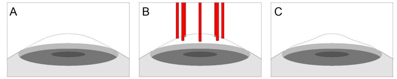
In this article we propose an alternative formulation to model a thermal-optical coupled problem involving laser heating. We show that by using the Fractional Beer-Lambert Law (FBLL) instead of the Beer-Lambert Law (BLL) as the governing equation of the optical problem, the formulation of the laser heat source changes, along with consequently, the distribution of temperatures. Our theoretical findings apply to laser thermal keratoplasty (LTK), used to reduce diopters of hyperopia. We show that the FBLL offers a new approach for heat conduction modeling of laser heating, which is more flexible and could better fit the data in cases where the BLL approach does not fit the data well. Our results can be extended to laser heating of other biological tissues and in other general applications. Our findings imply a new insight to improve the accuracy of thermal models, since they involve a new formulation of the external heat source rather than the heat equation itself.

References

[1]	I. Abdelhalim, O. Hamdy, A. A. Hassan, S. H. Elnaby, Dependence of the heating effect on tissue absorption coefficient during corneal reshaping using different UV lasers: A numerical study, Phys. Eng. Sci. Med. 44 (2021), 221–227. https://doi.org/10.1007/s13246-021-00971-x
[2]	A. E, Abouelregal, K. M. Khalil, W. W. Mohammed, D. Atta, Thermal vibration in rotating nanobeams with temperature–dependent due to exposure to laser irradiation, AIMS Math., 7 (2022), 6128–6152. https://doi.org/10.3934/math.2022341 doi: 10.3934/math.2022341
[3]	A. E. Abouelregal, A. Soleiman, H. M. Sedighi, K. M. Khalil, M. E. Nasr, Advanced thermoelastic heat conduction model with two fractional parameters and phase-lags, Phys. Scr., 96 (2021), 124048. https://doi.org/10.1088/1402-4896/ac2f80 doi: 10.1088/1402-4896/ac2f80
[4]	G. Casasanta, D. Ciani, R. Garra, Non-exponential extinction of radiation by fractional calculus modelling, J. Quant. Spectrosc. Radiat. Transf., 113 (2012), 194–197. https://doi.org/10.1016/j.jqsrt.2011.10.003 doi: 10.1016/j.jqsrt.2011.10.003
[5]	D. Fuente, C. Lizama, J. F. Urchueguía, J. A. Conejero, Estimation of the light field inside photosynthetic microorganism cultures through Mittag-Leffler functions at depleted light conditions, J. Quant. Spectrosc. Radiat. Transf., 204 (2018), 23–26. https://doi.org/10.1016/j.jqsrt.2017.08.012 doi: 10.1016/j.jqsrt.2017.08.012
[6]	M. Ghanbari, G. Rezazadeh, Thermo-vibrational analyses of skin tissue subjected to laser heating source in thermal therapy, Sci. Rep., 11 (2021), 22633. https://doi.org/10.1038/s41598-021-02006-7 doi: 10.1038/s41598-021-02006-7
[7]	A. L. Gough-Palmer, W. M. Gedroyc, Laser ablation of hepatocellular carcinoma–a review, World J. Gastroenterol., 14 (2008), 7170–7174. https://doi.org/10.3748/wjg.14.7170 doi: 10.3748/wjg.14.7170
[8]	P. Grigolini, A. Rocco, B. J. West, Fractional calculus as a macroscopic manifestation of randmoness, Phys. Rev. E., 59 (1999), 3. https://doi.org/10.1103/PhysRevE.59.2603 doi: 10.1103/PhysRevE.59.2603
[9]	C. Y. Hsiao, S. C. Yang, A. Alalaiwe, J. Y. Fang, Laser ablation and topical drug delivery: A review of recent advances, Expert. Opin. Drug. Deliv., 16 (2019), 937–952. https://doi.org/10.1080/17425247.2019.1649655 doi: 10.1080/17425247.2019.1649655
[10]	R. Ibrahim, C. Ozel, On Multi-Order fractional differential operators in the unit disk, Filomat, 30 (2016), 73–81. https://doi.org/10.2298/FIL1601073I doi: 10.2298/FIL1601073I
[11]	H. E. John, P. J. Mahaffey, Laser ablation and cryotherapy of melanoma metastases, J. Surg. Oncol., 109 (2014), 296–300. https://doi.org/10.1002/jso.23488 doi: 10.1002/jso.23488
[12]	A. Kabiri, M. R. Talaee, Thermal field and tissue damage analysis of moving laser in cancer thermal therapy, Lasers Med. Sci., 36 (2021), 583–597. https://doi.org/10.1007/s10103-020-03070-7 doi: 10.1007/s10103-020-03070-7
[13]	D. Kim, H. Kim, Induction of apoptotic temperature in photothermal therapy under various heating conditions in multi-layered skin structure, Int. J. Mol. Sci., 22 (2021), 11091. https://doi.org/10.3390/ijms222011091 doi: 10.3390/ijms222011091
[14]	A. N. Kochubei, Y. F. Luchko, Handbook of fractional calculus with applications, 1 (2019), 2019.
[15]	A. Liemert, A. Kienle, Radiative transport equation for the Mittag-Leffler path length distribution, J. Math. Phys., 58 (1017), 053511. https://doi.org/10.1063/1.4983682 doi: 10.1063/1.4983682
[16]	A. Liemert, A. Kienle, Fractional radiative transport in the diffusion approximation, J. Math. Chem., 2017. https://doi.org/10.1007/s10910-017-0792-2
[17]	R. R. Letfullin, S. A. Szatkowski, Laser-induced thermal ablation of cancerous cell organelles, Ther. Deliv., 8 (2017), 501–509. https://doi.org/10.4155/tde-2016-0087 doi: 10.4155/tde-2016-0087
[18]	C. Lizama, M. Trujillo, The time fractional approach for the modeling of thermal therapies: Temperature analysis in laser irradiation, Int. J. Heat Mass. Transfer., 154 (2020), 119677. https://doi.org/10.1016/j.ijheatmasstransfer.2020.119677 doi: 10.1016/j.ijheatmasstransfer.2020.119677
[19]	E. Luther, S. Mansour, N. Echeverry, D. McCarthy, D. G. Eichberg, A. Shah, et al., Laser ablation for cerebral metastases, Neurosurg. Clin. N. Am., 31 (2020), 537–547. https://doi.org/10.1016/j.nec.2020.06.004 doi: 10.1016/j.nec.2020.06.004
[20]	F. Manns, D. Borja, J. M. A. Parel, W. E. Smiddy, W. Culbertson, Semianalytical thermal model for subablative laser heating of homogeneous nonperfused biological tissue: Application to laser thermokeratoplasty, J. Biomed. Optics., 2003; 8 (2003), 288–297. https://doi.org/10.1117/1.1560644
[21]	A. Narasimhan, K. K. Jha, Bio-heat transfer simulation of retinal laser irradiation, Int. J. Numer. Method Biomed. Eng., 28 (2012), 547–559. https://doi.org/10.1002/cnm.1489
[22]	P. Ooshiar, A. Moradi, B. Khezry, Bioheat transfer analysis of biological tissues induced by laser irradiation, Int. J. Thermal. Sci., 90 (2015). https://doi.org/10.1016/j.ijthermalsci.2014.12.004
[23]	I. Oshina, J. Spigulis, Beer–Lambert law for optical tissue diagnostics: Current state of the art and the main limitations, J. Biomed. Optics., 26 (2021), 100901. https://doi.org/10.1117/1.JBO.26.10.100901 doi: 10.1117/1.JBO.26.10.100901
[24]	A. D. Poularikas, The Handbook of Formulas and Tables for Signal Processing, CRC Press LLC, 1999.
[25]	E. V. Ross, F. P. Sajben, J. Hsia, D. Barnette, C. H. Miller, J. R. McKinlay, Nonablative skin remodeling: Selective dermal heating with a mid-infrared laser and contact cooling combination, Lasers Surg. Med., 26 (2000), 186–195. https://doi.org/10.1002/(SICI)1096-9101(2000)26:2<186::AID-LSM9>3.0.CO;2-I doi: 10.1002/(SICI)1096-9101(2000)26:2<186::AID-LSM9>3.0.CO;2-I
[26]	F. Rossi, R. Pini, L. Menabuoni, Experimental and model analysis on the temperature dynamics during diode laser welding of the cornea, J. Biomed. Opt., 12 (2007), 014031. https://doi.org/10.1117/1.2437156 doi: 10.1117/1.2437156
[27]	M. Şen, A. E. Çalık, H. Ertik, Determination of half-value thickness of aluminum foils for different beta sources by using fractional calculus, Nucl. Instrum. Methods Phys. Res., 335 (2014), 78–84. https://doi.org/10.1016/j.nimb.2014.06.005 doi: 10.1016/j.nimb.2014.06.005
[28]	V. Tramontana, G. Casasanta, R. Garra, A. M. Iannarelli, An application of Wright functions to the photon propagation, J. Quant. Spectrosc. Radiat. Transf., 124 (2013), 45–48. https://doi.org/10.1016/j.jqsrt.2013.03.008 doi: 10.1016/j.jqsrt.2013.03.008
[29]	M. Trujillo, M. J. Rivera, J. A. Molina López, E. Berjano, Analytical thermal–optic model for laser heating of biological tissue using the hyperbolic heat transfer equation, Math. Med. Biol., 26 (2009), 187–200. https://doi.org/10.1093/imammb/dqp002 doi: 10.1093/imammb/dqp002
[30]	M. E. Vuylsteke, S. R. Mordon, Endovenous laser ablation: A review of mechanisms of action, Ann. Vasc. Surg., 26 (2012), 424–433. https://doi.org/10.1016/j.avsg.2011.05.037 doi: 10.1016/j.avsg.2011.05.037
[31]	J. N. Webb, H. Zhang, A. Sinha Roy, J. B. Randleman, G. Scarcelli, Detecting Mechanical Anisotropy of the Cornea Using Brillouin Microscopy, Transl. Vis. Sci. Technol., 9 (2020), 26. https://doi.org/10.1167/tvst.9.7.26 doi: 10.1167/tvst.9.7.26
[32]	K. Zhang, Y. Zhang, J. Li, Q. Wang, A contrastive analysis of laser heating between the human and guinea pig cochlea by numerical simulations, Biomed Eng Online., 15 (2016), 59. https://doi.org/10.1186/s12938-016-0190-1 doi: 10.1186/s12938-016-0190-1

Reader Comments

Your name:*

Email:*
© 2022 the Author(s), licensee AIMS Press. This is an open access article distributed under the terms of the Creative Commons Attribution License (http://creativecommons.org/licenses/by/4.0)