Effect of immigration in a predator-prey system: Stability, bifurcation and chaos

Figen Kangalgil; Seval Isșık; Figen Kangalgil; Seval Isșık

doi:10.3934/math.2022791

AIMS Mathematics

2022, Volume 7, Issue 8: 14354-14375. doi: 10.3934/math.2022791

Previous Article Next Article

Research article Special Issues

Effect of immigration in a predator-prey system: Stability, bifurcation and chaos

Figen Kangalgil ^{1
,
,},
Seval Isșık ^{2
,
,}

1.
Bergama Vocational School, Dokuz Eylul University, Izmir 35700, Turkey
2.
Department of Mathematics and Science Education, Faculty of Education, Sivas Cumhuriyet University, Sivas 58140, Turkey

Received: 30 December 2021 Revised: 07 May 2022 Accepted: 09 May 2022 Published: 02 June 2022
MSC : 39A33, 37G35, 39A30

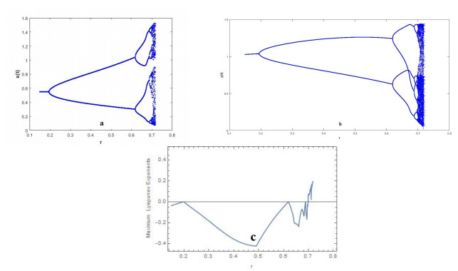
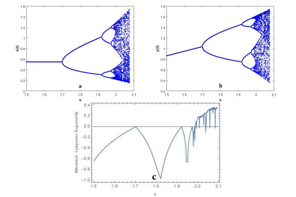
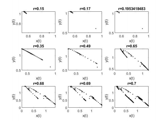
In the present manuscript, a discrete-time predator-prey system with prey immigration is considered. The existence of the possible fixed points of the system and topological classification of coexistence fixed point are analyzed. Moreover, the existence and the direction for both Neimark-Sacker bifurcation and flip bifurcation are investigated by applying bifurcation theory. In order to control chaos due to the emergence of the Neimark-Sacker bifurcation, an OGY feedback control strategy is implemented. Furthermore, some numerical simulations, including bifurcation diagrams, phase portraits and maximum Lyapunov exponents of the system, are given to support the accuracy of the analytical finding. The computation of the maximum Lyapunov exponents confirms the presence of chaotic behavior in the system.
- predator-prey system,
- fixed point,
- stability,
- immigration,
- Neimark-Sacker bifurcation,
- flip bifurcation,
- chaotic behavior,
- OGY feedback control method
Citation: Figen Kangalgil, Seval Isșık. Effect of immigration in a predator-prey system: Stability, bifurcation and chaos[J]. AIMS Mathematics, 2022, 7(8): 14354-14375. doi: 10.3934/math.2022791

Related Papers:

Abstract

In the present manuscript, a discrete-time predator-prey system with prey immigration is considered. The existence of the possible fixed points of the system and topological classification of coexistence fixed point are analyzed. Moreover, the existence and the direction for both Neimark-Sacker bifurcation and flip bifurcation are investigated by applying bifurcation theory. In order to control chaos due to the emergence of the Neimark-Sacker bifurcation, an OGY feedback control strategy is implemented. Furthermore, some numerical simulations, including bifurcation diagrams, phase portraits and maximum Lyapunov exponents of the system, are given to support the accuracy of the analytical finding. The computation of the maximum Lyapunov exponents confirms the presence of chaotic behavior in the system.

References

[1]	A. J. Lotka, Elements of mathematical biology, Williams & Wilkins, Baltimore, 1925.
[2]	V. Volterra, Variazioni e fluttuazioni del numero d'individui in specie animali conviventi, Memoire della R. Accad. Nazionale dei Lincei, 1926.
[3]	V. Krivan, Prey-predator models, In: S. E. Jørgensen, B. D. Fath, Encyclopedia of ecology, 4 (2008), 2929–2940.
[4]	U. Ufuktepe, S. Kapçak, O. Akman, Stability analysis of the Beddington model with Allee effect, Appl. Math. Inf. Sci., 9 (2015), 603–608.
[5]	U. Ufuktepe, S. Kapcak, Generalized Beddington model with the host subject to the Allee effect, Open Phys., 13 (2015), 428–434. https://doi.org/10.1515/phys-2015-0055 doi: 10.1515/phys-2015-0055
[6]	H. I. McCallum, Effects of immigration on chaotic population dynamics, J. Theor. Biol., 154 (1992), 277–284. https://doi.org/10.1016/S0022-5193(05)80170-5 doi: 10.1016/S0022-5193(05)80170-5
[7]	S. Işık, A study of stability and bifurcation analysis in discrete-time predator-prey system involving the Allee effect, Int. J. Biomath., 12 (2019), 1950011. https://doi.org/10.1142/S1793524519500116 doi: 10.1142/S1793524519500116
[8]	Q. Din, Neimark-Sacker bifurcation and chaos control in Hassel-Varley model, J. Differ. Equ. Appl., 23 (2016), 741–762. https://doi.org/10.1080/10236198.2016.1277213 doi: 10.1080/10236198.2016.1277213
[9]	Q. Din, Complexity and choas control in a discrete-time prey-predator model, Commun. Nonlinear Sci. Numer. Simul., 49 (2017), 113–134. https://doi.org/10.1016/j.cnsns.2017.01.025 doi: 10.1016/j.cnsns.2017.01.025
[10]	Q. Din, Controlling chaos in a discrete-time prey-predator model with Allee effects, Int. J. Dyn. Control, 6 (2018), 858–872. https://doi.org/10.1007/s40435-017-0347-1 doi: 10.1007/s40435-017-0347-1
[11]	O. A. Gumus, F. Kangalgil, Dynamics of a host-parasite model connected with immigration, New Trends Math. Sci., 5 (2017), 332–339.
[12]	R. D. Holt, Immigration and the dynamics of peripheral populations, Advances in Herpetology and Evolutionary Biology, Harvard University, Cambridge, 1983.
[13]	S. Kartal, Mathematical modeling and analysis of tumor-immune system interastion by using Lotka-Volterra predator-prey like model with piecewise constant arguments, Period. Eng. Nat. Sci., 2 (2014), 7–12. http://dx.doi.org/10.21533/pen.v2i1.36 doi: 10.21533/pen.v2i1.36
[14]	S. Kartal, Dynamics of a plant-herbivore model with differential-difference equations, Cogent Math., 3 (2016), 1136198. https://doi.org/10.1080/23311835.2015.1136198 doi: 10.1080/23311835.2015.1136198
[15]	S. Kartal, Flip and Neimark-Sacker bifurcation in a differential equation with piecewise constant arguments model, J. Differ. Equ. Appl., 23 (2017), 763–778. https://doi.org/10.1080/10236198.2016.1277214 doi: 10.1080/10236198.2016.1277214
[16]	S. Kartal, F. Gurcan, Global behaviour of a predator-prey like model with piecewise constant arguments, J. Biol. Dyn., 9 (2015), 159–171. https://doi.org/10.1080/17513758.2015.1049225 doi: 10.1080/17513758.2015.1049225
[17]	R. Yang, J. Dan, W. Wenlog, A diffusive predator-prey model with generalist predator and time delay, AIMS Math., 7 (2022), 4574–4591. https://doi.org/10.3934/math.2022255 doi: 10.3934/math.2022255
[18]	A. Q. Khan, Neimark-Sacker bifurcation of a two-dimensional discrete-time predator-prey model, SpringerPlus, 5 (2016), 126. https://doi.org/10.1186/s40064-015-1618-y doi: 10.1186/s40064-015-1618-y
[19]	A. Q. Khan, Stability and Neimark-Sacker bifurcation of a ratio-dependence predator-prey model, Math. Methods Appl. Sci., 40 (2017), 4109–4117. https://doi.org/10.1002/mma.4290 doi: 10.1002/mma.4290
[20]	R. K. Ghaziani, W. Govaerts, C. Sonck, Resonance and bifurcation in a discrete-time predator-prey system with Holling functional response, Nonlinear Anal.: Real World Appl., 13 (2012), 1451–1465. https://doi.org/10.1016/j.nonrwa.2011.11.009 doi: 10.1016/j.nonrwa.2011.11.009
[21]	Y. A. Kuznetsov, Elements of applied bifurcation theory, New York: Springer-Verlag, 1998.
[22]	E. Ott, C. Grebogi, J. A. Yorke, Controlling choas, Phys. Rev. Lett., 64 (1990), 1196–1199. https://doi.org/10.1103/PhysRevLett.64.1196 doi: 10.1103/PhysRevLett.64.1196
[23]	S. M. S. Rana, Bifurcation and complex dynamics of a discrete-time predator-prey system, Comput. Ecol. Software, 5 (2015), 187–200.
[24]	S. M. S. Rana, U. Kulsum, Bifurcation analysis and chaos control in a discrete-time predator-prey system of Leslie type with simplified Holling type Ⅳ functional response, Discrete Dyn. Nature Soc., 2017 (2017), 9705985. https://doi.org/10.1155/2017/9705985 doi: 10.1155/2017/9705985
[25]	S. M. S. Rana, Bifurcation and complex dynamics of a discrete-time predator-prey system involving roup defense, Comput. Ecol. Software, 5 (2015), 222–238.
[26]	J. Sugie, Y. Saito, Uniqueness of limit cycles in a Rosenzweig-Macarthur model with prey immigration, SIAM J. Appl. Math., 72 (2012), 299–316. https://doi.org/10.1137/11084008X doi: 10.1137/11084008X
[27]	G. Zhu, J. Wei, Global stability and bifurcation analysis of a delayed predator-prey system with prey immigration, Electron. J. Qual. Theory Differ. Equ., 13 (2016), 1–20.
[28]	I. Seval, F. Kangalgil, On the analysis of stability, bifurcation, and chaos control of discrete-time predator-prey model with Allee effect on predator, Hacettepe J. Math. Stat., 51 (2022), 404–420.
[29]	M. A. Stephano, I. H. Jung, Effects of refuge prey on stability of the prey-predator model subject to immigrants: A mathematical modelling approach, Tanzania J. Sci., 47 (2021), 1376–1391.
[30]	P. Rohani, O. Miramontes, Immigration and the persistence of chaos in population models, J. Theor. Biol., 175 (1995), 203–206. https://doi.org/10.1006/jtbi.1995.0133 doi: 10.1006/jtbi.1995.0133
[31]	G. D. Ruxton, Low levels of immigration between chaotic populations can reduce system extinctions by inducing asynchronous regular cycles, Proc. Royal Soc. London B, 256 (1994), 189–193. https://doi.org/10.1098/rspb.1994.0069 doi: 10.1098/rspb.1994.0069
[32]	L. Stone, D. Hart, Effects of immigration on dynamics of simple population models, Theor. Popul. Biol., 55 (1999), 227–234. https://doi.org/10.1006/tpbi.1998.1393 doi: 10.1006/tpbi.1998.1393
[33]	F. Kangalgil, N. Topsakal, Stability analysis and flip bifurcation of a discrete-time prey-predator model with predator immigration, Asian J. Math. Comput. Res., 27 (2020), 1–10.
[34]	F. Kangalgil, F. Gümüşboğa, Period-doubling bifurcation and stability in a two dimensional discrete prey-predator model with Allee effect and immigration parameter on prey, Cumhuriyet Sci. J., 43 (2022), 88–97. https://doi.org/10.17776/csj.1026330 doi: 10.17776/csj.1026330
[35]	L. Stone, Period-doubling reversals and chaos in simple ecological model, Nature, 365 (1993), 617–620. https://doi.org/10.1038/365617a0 doi: 10.1038/365617a0
[36]	T. Tahara, M. K. A. Gavina, T. Kawano, J. M. Tubay, J. F. Rabajante, H. Ito, et al., Asymptotic stability of a modified Lotka-Volterra model with small immigrations, Sci. Rep., 8 (2018), 7029. https://doi.org/10.1038/s41598-018-25436-2 doi: 10.1038/s41598-018-25436-2
[37]	S. Wiggins, Introduction to applied nonlinear dynamical system and chaos, New York: Springer-Verlag, 2003.
[38]	G. P. Neverova, O. L. Zhnadova, B. Ghosh, E. Y Frisman, Dynamics of a discrete-time stage-structured predator-prey system with Holling type Ⅱ response function, Nonlinear Dyn., 98 (2019), 427–446. https://doi.org/10.1007/s11071-019-05202-3 doi: 10.1007/s11071-019-05202-3

Reader Comments

Your name:*

Email:*
© 2022 the Author(s), licensee AIMS Press. This is an open access article distributed under the terms of the Creative Commons Attribution License (http://creativecommons.org/licenses/by/4.0)