The exact solutions of conformable time-fractional modified nonlinear Schrödinger equation by Direct algebraic method and Sine-Gordon expansion method

Safoura Rezaei Aderyani; Reza Saadati; Javad Vahidi; Nabil Mlaiki; Thabet Abdeljawad; Safoura Rezaei Aderyani; Reza Saadati; Javad Vahidi; Nabil Mlaiki; Thabet Abdeljawad

doi:10.3934/math.2022604

AIMS Mathematics

2022, Volume 7, Issue 6: 10807-10827. doi: 10.3934/math.2022604

Previous Article Next Article

Research article Special Issues

The exact solutions of conformable time-fractional modified nonlinear Schrödinger equation by Direct algebraic method and Sine-Gordon expansion method

1.
School of Mathematics, Iran University of Science and Technology, Narmak, Tehran, Iran
2.
Department of Mathematics and Sciences, Prince Sultan University, P.O. Box 66833, 11586 Riyadh, Saudi Arabia
3.
Department of Medical Research, China Medical University, Taichung 40402, Taiwan

Received: 14 December 2021 Revised: 01 March 2022 Accepted: 07 March 2022 Published: 31 March 2022
MSC : 35C07, 35C08, 35G50, 35Q60, 35R11, 65H10

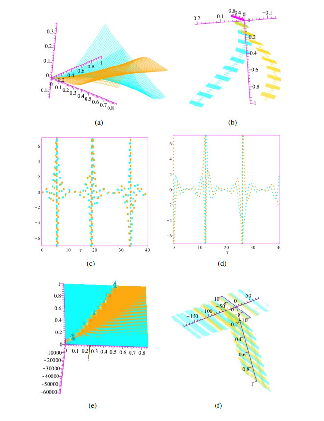
In this article, we used direct algebraic method (DAM) and sine-Gordon expansion method (SGEM), to find the analytical solutions of conformable time-fractional modified nonlinear Schrödinger equation (CTFMNLSE) and finally, we present numerical results in tables and charts.

Keywords:

Citation: Safoura Rezaei Aderyani, Reza Saadati, Javad Vahidi, Nabil Mlaiki, Thabet Abdeljawad. The exact solutions of conformable time-fractional modified nonlinear Schrödinger equation by Direct algebraic method and Sine-Gordon expansion method[J]. AIMS Mathematics, 2022, 7(6): 10807-10827. doi: 10.3934/math.2022604

Related Papers:

[1]	Yaya Wang, Md Nurul Raihen, Esin Ilhan, Haci Mehmet Baskonus . On the new sine-Gordon solitons of the generalized Korteweg-de Vries and modified Korteweg-de Vries models via beta operator. AIMS Mathematics, 2025, 10(3): 5456-5479. doi: 10.3934/math.2025252
[2]	Wei Gao, Gulnur Yel, Haci Mehmet Baskonus, Carlo Cattani . Complex solitons in the conformable (2+1)-dimensional Ablowitz-Kaup-Newell-Segur equation. AIMS Mathematics, 2020, 5(1): 507-521. doi: 10.3934/math.2020034
[3]	Zeliha Korpinar, Mustafa Inc, Ali S. Alshomrani, Dumitru Baleanu . The deterministic and stochastic solutions of the Schrodinger equation with time conformable derivative in birefrigent fibers. AIMS Mathematics, 2020, 5(3): 2326-2345. doi: 10.3934/math.2020154
[4]	M. Ali Akbar, Norhashidah Hj. Mohd. Ali, M. Tarikul Islam . Multiple closed form solutions to some fractional order nonlinear evolution equations in physics and plasma physics. AIMS Mathematics, 2019, 4(3): 397-411. doi: 10.3934/math.2019.3.397
[5]	Mustafa Inc, Hadi Rezazadeh, Javad Vahidi, Mostafa Eslami, Mehmet Ali Akinlar, Muhammad Nasir Ali, Yu-Ming Chu . New solitary wave solutions for the conformable Klein-Gordon equation with quantic nonlinearity. AIMS Mathematics, 2020, 5(6): 6972-6984. doi: 10.3934/math.2020447
[6]	M. Hafiz Uddin, M. Ali Akbar, Md. Ashrafuzzaman Khan, Md. Abdul Haque . New exact solitary wave solutions to the space-time fractional differential equations with conformable derivative. AIMS Mathematics, 2019, 4(2): 199-214. doi: 10.3934/math.2019.2.199
[7]	Abdullahi Yusuf, Tukur A. Sulaiman, Mustafa Inc, Sayed Abdel-Khalek, K. H. Mahmoud . $M-$ truncated optical soliton and their characteristics to a nonlinear equation governing the certain instabilities of modulated wave trains. AIMS Mathematics, 2021, 6(9): 9207-9221. doi: 10.3934/math.2021535
[8]	M. TarikulIslam, M. AliAkbar, M. Abul Kalam Azad . Traveling wave solutions in closed form for some nonlinear fractional evolution equations related to conformable fractional derivative. AIMS Mathematics, 2018, 3(4): 625-646. doi: 10.3934/Math.2018.4.625
[9]	Xiaoli Wang, Lizhen Wang . Traveling wave solutions of conformable time fractional Burgers type equations. AIMS Mathematics, 2021, 6(7): 7266-7284. doi: 10.3934/math.2021426
[10]	Amir Ali, Abid Ullah Khan, Obaid Algahtani, Sayed Saifullah . Semi-analytical and numerical computation of fractal-fractional sine-Gordon equation with non-singular kernels. AIMS Mathematics, 2022, 7(8): 14975-14990. doi: 10.3934/math.2022820

Abstract

1. Introduction

The notion of fractional derivative (FD) is more than three thousand years old, the role of fractional calculus has been increasing due to its application zone in various domains including biology, semiconductor industry, optical communication, energy quantization, quantum chemistry, wave propagation, protein folding and bending, condensed matter physics, solid state physics, nanotechnology and industry, laser propagation, nonlinear optics etc. the fractional differential equations (FDEs), have received a great deal of interest from scholars and researchers. Many mathematicians presented diverse types of FDs, such as that given in ^[1,2]. The most famous ones are Hadamard, Marchaud, Riemann-Liouville, Grunwald-Letnikov, Kober, Caputo, Riesz and Erdelyi.

Lately, a novel FD has been presented by Khalil et al. ^[3] and others ^[4,5,6], called conformable FD. Due to the significance of the exact solutions of NLSEs, plenty of mathematicians solved them with conformable derivative, who used the different methods like first integral method (FIM) ^[7,8], functional variable method (FVM) ^[7,9], trial equation method (TEM) ^[10], modified trial equation method (MTEM) ^[11], direct algebraic method (DAM) ^[12] and sine-Gordon expansion method (SGEM) ^[13] to find the exact solutions to NLSEs.

In ^[14], Younas et al. presented CTFMNLSE and studied the exact solutions of it by the generalized exponential rational function method. Also in ^[15,16], authors introduced some new solutions of CTFMNLSE via FIM, FVM, TEM and MTEM.

Motivated by the work done in ^[14,15,16], we consider the following CTFMNLSE:

$\begin{equation} \text{i}\mathbf{D}^{\alpha}_{\tau}\Psi+\sigma_{1} \Psi_{\mathfrak{X}\mathfrak{X}}+\sigma_{2} \vert \Psi \vert^{2}\Psi = \text{i}\delta_{1}\Psi_{\mathfrak{X}\mathfrak{X}\mathfrak{X}}+\text{i}\delta_{2} \Psi^{2}\Psi_{\mathfrak{X}}^{*}-\text{i}\delta_{3} \vert \Psi \vert^{2}\Psi_{\mathfrak{X}}+\delta_{4}\Psi \:\:\:\:\:\:\:\: 0 < \alpha\leq 1, \end{equation}$

(1.1)

where $\sigma_{1} = \dfrac{\mathcal{P}_{0}}{8\mathcal{K}_{0}^{2}(-3\cos(\Theta)+2)}$ , $\sigma_{2} = \dfrac{-\mathcal{P}_{0}\mathcal{K}_{0}^{2}}{2}$ , $\delta_{1} = \dfrac{\mathcal{P}_{0}\cos(\Theta)}{16\mathcal{K}_{0}^{3}(-5\cos^{2}(\Theta)-6)}$ , $\delta_{2} = \dfrac{\mathcal{P}_{0}\mathcal{K}_{0}\cos(\Theta)}{4}$ , $\delta_{3} = \dfrac{3\mathcal{P}_{0}\mathcal{K}_{0}}{2}, \delta_{4} = \mathcal{K}_{0}\vert \Psi \vert^{2}_{\mathfrak{X}} \bigg\vert_{\mathfrak{X} = 0}$ , $\mathcal{P}_{0}$ and $\mathcal{K}_{0}$ are the frequency and the wave number of the carrier wave, respectively, and the operator $\mathbf{D}^{\alpha}$ of order $\alpha$ , where $\alpha\in(0, 1]$ represents the conformable fractional derivative.

2. Preliminaries

In this section, we present some properties and definitions of the conformal derivative and other Preliminaries.

Definition 2.1. ^[3] Suppose $\Omega : (0, \infty) \rightarrow \mathbb{R}$ is a function. Therefore the conformal fractional derivative of $\Omega$ of order $\alpha$ is as follows

$\begin{equation} \mathbf{T}_{\alpha}(\tau) = \lim\limits_{\epsilon\rightarrow 0 } \dfrac{\Omega (\tau+\epsilon \tau^{1-\alpha})-\Omega(\tau)}{\epsilon} \end{equation}$

(2.1)

for all $0 < \alpha < 1, 0 < \tau$ .

Definition 2.2. ^[3] Suppose $\iota\geq 0$ and $\tau \geq \iota$ . Also, suppose $\Omega$ is a function defined on $(\iota, \tau]$ and $\alpha \in \mathbb{R}$ . Therefore, the $\alpha$ -fractional integral of $\Omega$ is defined by,

$\begin{equation} \mathbf{I}_{\iota}^{\alpha}\Omega(\tau) = \int_{\iota}^{\tau}\dfrac{\Omega(\varsigma)}{\varsigma^{1-\alpha}}d\varsigma, \end{equation}$

(2.2)

if the Riemann improper integral exists.

Theorem 2.3. ^[3]Suppose $0 < \alpha \leq 1$ , and $\Omega$ and $\mho$ are $\alpha-$ differentiable at a point $\tau$ , therefore

(i) $\mathbf{T}_{\alpha}(\varpi_{1}\Omega+\varpi_{2} \mho) = \varpi_{1} \mathbf{T}_{\alpha}(\Omega)+\varpi_{2} \mathbf{T}_{\alpha}(\mho), \:\: \forall \varpi_{1}, \varpi_{2}\in \mathbb{R}$ .

(ii) $\mathbf{T}_{\alpha}(t^{\varpi}) = \varpi \tau^{\varpi-\alpha}, \:\:\forall \varpi\in \mathbb{R}$ .

(iii) ${}_{\tau}\mathbf{T}_{\alpha}(\Omega\mho) = \Omega \mathbf{T}_{\alpha}(\mho)+\mho\mathbf{T}_{\alpha}(\Omega)$ .

(iv) $\mathbf{T}_{\alpha}\bigg(\dfrac{\Omega}{\mho}\bigg) = \dfrac{\mho\mathbf{T}_{\alpha}(\Omega)-\Omega\mathbf{T}_{\alpha}(\mho)}{\mho^{2}}$ .

Furthermore, if $\Omega$ is differentiable, then $\mathbf{T}_{\alpha}(\Omega)(\tau) = \tau^{1-\alpha}\dfrac{d\Omega}{d\tau}$ .

Theorem 2.4. ^[3] Suppose $\Omega:(0, \infty)\rightarrow \mathbb{R}$ is a function s.t. $\Omega$ is differentiable and also $\alpha$ -differentiable. Suppose $\mho$ is a function defined in the range of $\Omega$ and also differentiable; therefore, one has the following rule

$\mathbf{T}_{\alpha}(\Omega \mathit{\text{o}} \: \mho) (\tau) = \tau^{1-\alpha} \mho(\tau)\Omega^{\prime} (\mho(\tau)).$

Remark 2.5. Let

$\begin{equation} \mathcal{Q}^{\prime}(\xi) = \text{Ln} (A)(\mathfrak{P}_{0}+\mathfrak{P}_{1}\mathcal{Q}(\xi)+\mathfrak{P}_{2}\mathcal{Q}^{2}(\xi)), \:\:\:\:\:\:A\neq 0, 1. \end{equation}$

(2.3)

The solutions of ODE (2.3) are:

(1) When $\mathfrak{P}^{2}_{1} - 4\mathfrak{P}_{0} \mathfrak{P}_{2} < 0$ and $\mathfrak{P}_{2}\neq 0,$

$\begin{equation*} \mathcal{Q}_{1}(\xi) = -\dfrac{\mathfrak{P}_{1}}{2\mathfrak{P}_{2}}+\dfrac{\sqrt{-( \mathfrak{P}^{2}_{1} - 4\mathfrak{P}_{0} \mathfrak{P}_{2})}}{2\mathfrak{P}_{2}}\text{tan}_{A}\bigg( \dfrac{\sqrt{-( \mathfrak{P}^{2}_{1} - 4\mathfrak{P}_{0} \mathfrak{P}_{2})}}{2}\xi \bigg), \end{equation*}$

$\begin{equation*} \mathcal{Q}_{2}(\xi) = -\dfrac{\mathfrak{P}_{1}}{2\mathfrak{P}_{2}}-\dfrac{\sqrt{-( \mathfrak{P}^{2}_{1} - 4\mathfrak{P}_{0} \mathfrak{P}_{2})}}{2\mathfrak{P}_{2}}\text{cot}_{A}\bigg( \dfrac{\sqrt{-( \mathfrak{P}^{2}_{1} - 4\mathfrak{P}_{0} \mathfrak{P}_{2})}}{2}\xi \bigg), \end{equation*}$

$\begin{eqnarray*} \mathcal{Q}_{3}(\xi)& = &-\dfrac{\mathfrak{P}_{1}}{2\mathfrak{P}_{2}}+\dfrac{\sqrt{-( \mathfrak{P}^{2}_{1} - 4\mathfrak{P}_{0} \mathfrak{P}_{2})}}{2\mathfrak{P}_{2}}\text{tan}_{A}( \sqrt{-( \mathfrak{P}^{2}_{1} - 4\mathfrak{P}_{0} \mathfrak{P}_{2})}\xi )\\ &\pm &\notag\dfrac{\sqrt{-sr ( \mathfrak{P}^{2}_{1} - 4\mathfrak{P}_{0} \mathfrak{P}_{2})}}{2\mathfrak{P}_{2}}\text{sec}_{A}( \sqrt{-( \mathfrak{P}^{2}_{1} - 4\mathfrak{P}_{0} \mathfrak{P}_{2})}\xi ), \end{eqnarray*}$

$\begin{eqnarray*} \mathcal{Q}_{4}(\xi)& = &-\dfrac{\mathfrak{P}_{1}}{2\mathfrak{P}_{2}}-\dfrac{\sqrt{-( \mathfrak{P}^{2}_{1} - 4\mathfrak{P}_{0} \mathfrak{P}_{2})}}{2\mathfrak{P}_{2}}\text{cot}_{A}( \sqrt{-( \mathfrak{P}^{2}_{1} - 4\mathfrak{P}_{0} \mathfrak{P}_{2})}\xi )\\ &\pm &\notag\dfrac{\sqrt{-sr ( \mathfrak{P}^{2}_{1} - 4\mathfrak{P}_{0} \mathfrak{P}_{2})}}{2\mathfrak{P}_{2}}\text{csc}_{A}( \sqrt{-( \mathfrak{P}^{2}_{1} - 4\mathfrak{P}_{0} \mathfrak{P}_{2})}\xi ), \end{eqnarray*}$

$\begin{eqnarray*} \mathcal{Q}_{5}(\xi)& = &-\dfrac{\mathfrak{P}_{1}}{2\mathfrak{P}_{2}}+\dfrac{\sqrt{-( \mathfrak{P}^{2}_{1} - 4\mathfrak{P}_{0} \mathfrak{P}_{2})}}{4\mathfrak{P}_{2}}\text{tan}_{A}( \dfrac{ \sqrt{-( \mathfrak{P}^{2}_{1} - 4\mathfrak{P}_{0} \mathfrak{P}_{2})}}{4}\xi )\\ &- &\notag\dfrac{\sqrt{- ( \mathfrak{P}^{2}_{1} - 4\mathfrak{P}_{0} \mathfrak{P}_{2})}}{4\mathfrak{P}_{2}}\text{cot}_{A}( \dfrac{ \sqrt{-( \mathfrak{P}^{2}_{1} - 4\mathfrak{P}_{0} \mathfrak{P}_{2})}}{4}\xi ), \end{eqnarray*}$

(2) When $\mathfrak{P}^{2}_{1} - 4\mathfrak{P}_{0} \mathfrak{P}_{2} > 0$ and $\mathfrak{P}_{2}\neq 0,$

$\begin{equation*} \mathcal{Q}_{6}(\xi) = -\dfrac{\mathfrak{P}_{1}}{2\mathfrak{P}_{2}}-\dfrac{\sqrt{\mathfrak{P}^{2}_{1} - 4\mathfrak{P}_{0} \mathfrak{P}_{2}}}{2\mathfrak{P}_{2}}\text{tanh}_{A}\bigg( \dfrac{\sqrt{ \mathfrak{P}^{2}_{1} - 4\mathfrak{P}_{0} \mathfrak{P}_{2}}}{2}\xi \bigg), \end{equation*}$

$\begin{equation*} \mathcal{Q}_{7}(\xi) = -\dfrac{\mathfrak{P}_{1}}{2\mathfrak{P}_{2}}-\dfrac{\sqrt{ \mathfrak{P}^{2}_{1} - 4\mathfrak{P}_{0} \mathfrak{P}_{2}}}{2\mathfrak{P}_{2}}\text{coth}_{A}\bigg( \dfrac{\sqrt{\mathfrak{P}^{2}_{1} - 4\mathfrak{P}_{0} \mathfrak{P}_{2}}}{2}\xi \bigg), \end{equation*}$

$\begin{eqnarray*} \mathcal{Q}_{8}(\xi)& = &-\dfrac{\mathfrak{P}_{1}}{2\mathfrak{P}_{2}}-\dfrac{\sqrt{ \mathfrak{P}^{2}_{1} - 4\mathfrak{P}_{0} \mathfrak{P}_{2}}}{2\mathfrak{P}_{2}}\text{tanh}_{A}( \sqrt{ \mathfrak{P}^{2}_{1} - 4\mathfrak{P}_{0} \mathfrak{P}_{2}}\xi )\\ &\pm &\notag\text{i}\dfrac{\sqrt{sr ( \mathfrak{P}^{2}_{1} - 4\mathfrak{P}_{0} \mathfrak{P}_{2})}}{2\mathfrak{P}_{2}}\text{sech}_{A}( \sqrt{\mathfrak{P}^{2}_{1} - 4\mathfrak{P}_{0} \mathfrak{P}_{2}}\xi ), \end{eqnarray*}$

$\begin{eqnarray*} \mathcal{Q}_{9}(\xi)& = &-\dfrac{\mathfrak{P}_{1}}{2\mathfrak{P}_{2}}-\dfrac{\sqrt{ \mathfrak{P}^{2}_{1} - 4\mathfrak{P}_{0} \mathfrak{P}_{2}}}{2\mathfrak{P}_{2}}\text{coth}_{A}( \sqrt{ \mathfrak{P}^{2}_{1} - 4\mathfrak{P}_{0} \mathfrak{P}_{2}}\xi )\\ &\pm &\notag\dfrac{\sqrt{sr( \mathfrak{P}^{2}_{1} - 4\mathfrak{P}_{0} \mathfrak{P}_{2})}}{2\mathfrak{P}_{2}}\text{csch}_{A}( \sqrt{ \mathfrak{P}^{2}_{1} - 4\mathfrak{P}_{0} \mathfrak{P}_{2}}\xi ), \end{eqnarray*}$

$\begin{eqnarray*} \mathcal{Q}_{10}(\xi)& = &-\dfrac{\mathfrak{P}_{1}}{2\mathfrak{P}_{2}}-\dfrac{\sqrt{ \mathfrak{P}^{2}_{1} - 4\mathfrak{P}_{0} \mathfrak{P}_{2}}}{4\mathfrak{P}_{2}}\text{tanh}_{A}( \dfrac{ \sqrt{ \mathfrak{P}^{2}_{1} - 4\mathfrak{P}_{0} \mathfrak{P}_{2}}}{4}\xi )\\ &- &\notag\dfrac{\sqrt{\mathfrak{P}^{2}_{1} - 4\mathfrak{P}_{0} \mathfrak{P}_{2}}}{4\mathfrak{P}_{2}}\text{coth}_{A}( \dfrac{ \sqrt{\mathfrak{P}^{2}_{1} - 4\mathfrak{P}_{0} \mathfrak{P}_{2}}}{4}\xi ), \end{eqnarray*}$

where generalized hyperbolic and triangular functions are given by

$\text{cosh}_{A}(\theta) = \dfrac{s A^{\theta}+r A^{-\theta}}{2}, \:\:\:\:\:\:\text{sinh}_{A}(\theta) = \dfrac{s A^{\theta}-r A^{-\theta}}{2},$

$\text{coth}_{A}(\theta) = \dfrac{s A^{\theta}+r A^{-\theta}}{s \text{e}^{\theta}-r\text{e}^{-\theta}}, \:\:\:\:\:\: \text{tanh}_{A}(\theta) = \dfrac{s A^{\theta}-r A^{-\theta}}{s \text{e}^{\theta}+r\text{e}^{-\theta}},$

$\text{csch}_{A}(\theta) = \dfrac{2}{s A^{\theta}-r A^{-\theta}}, \:\:\:\:\:\:\text{sech}_{A}(\theta) = \dfrac{2}{s A^{\theta}+rA^{-\theta}},$

$\text{cos}_{A}(\theta) = \dfrac{s A^{\text{i}\theta}+r A^{-\text{i}\theta}}{2\text{i}}, \:\:\:\:\:\:\text{sin}_{A}(\theta) = \dfrac{s A^{\text{i}\theta}-r A^{-\text{i}\theta}}{2\text{i}} ,$

$\text{cot}_{A}(\theta) = \text{i}\dfrac{s A^{\text{i}\theta}+r A^{-\text{i}\theta}}{s A^{\text{i}\theta}-r A^{-\text{i}\theta}}, \:\:\:\:\:\:\text{tan}_{A} (\theta) = -\text{i}\dfrac{s A^{\text{i}\theta}-r A^{-\text{i}\theta}}{s A^{\text{i}\theta}+r A^{-\text{i}\theta}},$

$\text{csc}_{A} (\theta) = \dfrac{2\text{i}}{s A^{\text{i}\theta}-r A^{-\text{i}\theta}}, \:\:\:\:\:\:\:\:\:\text{sec}_{A}(\theta) = \dfrac{2}{s A^{\text{i}\theta}+r A^{-\text{i}\theta}}, \:\:\:\:\:$

where $\theta$ is an independent variable, $A\neq 0, 1,$ and $s$ and $r$ are arbitrary constants greater than zero and are called deformation parameters.

3. Methods and applications

In this section, we present the first step of the DAM and the SGEM, for finding analytical solutions of CTFMNLSE defined as (1.1). Suppose a CTFNLPDE,

$\begin{equation} \Gamma \bigg(\Phi , \Phi_{\tau}, \Phi_{\mathfrak{X}}, \mathbf{D}_{\tau}^{\alpha}\Phi , \mathbf{D}_{\mathfrak{X}}^{\beta}\Phi , \mathbf{D}_{\tau}^{2\alpha}, \mathbf{D}_{\mathfrak{X}}^{2\beta}, \ldots\bigg) = 0, \:\:\:\:\:\:0 < \alpha, \beta\leq 1, \end{equation}$

(3.1)

where $\Gamma$ and $\Phi$ are a polynomial and an unknown function in its arguments, respectively. Using a fractional travelling wave transformation

$\begin{equation} \Phi (\mathfrak{X}, \tau) = \Lambda(\xi), \:\:\:\:\:\:\:\: \xi = \mathfrak{X}-\dfrac{\mathcal{V}}{\alpha}\tau^{\alpha} \end{equation}$

(3.2)

where $\mathcal{V}$ is velocity and substituting (3.2) into (3.1), we have a NLODE given by

$\begin{equation} \Upsilon (\Lambda , \Lambda^{\prime}, \Lambda^{\prime\prime}, \Lambda^{\prime\prime\prime}, \ldots) = 0, \end{equation}$

(3.3)

in which ${}^{\prime}$ signifies the derivative with respect to $\xi$ .

Since $\Psi = \Psi(\mathfrak{X}, \tau)$ in (1.1) is a complex function, we begin with the following travelling wave assumption

$\begin{equation} \Psi(\mathfrak{X}, \tau) = \Lambda(\xi)\text{e}^{\text{i}\psi} \end{equation}$

(3.4)

where $\xi = \eta (\mathfrak{X} - \dfrac{\mathcal{V}}{\alpha}\tau^{\alpha})$ and $\psi = -\mathcal{K}\mathfrak{X}+ \dfrac{\mathcal{P}}{\alpha}\tau^{\alpha}+\zeta$ , and $\zeta, \mathcal{P}$ and $\mathcal{K}$ are parameters, represent the phase constant, frequency and wave number respectively. Substitute (3.4) into (1.1), we get real and imaginary parts as follows

$\begin{equation} \eta^{2}(\sigma_{1}-3\delta_{1}\mathcal{K})\Lambda^{\prime\prime}+(\sigma_{2}+(\delta_{2}+\delta_{3})\mathcal{K})\Lambda^{3}+(-\mathcal{P} -\sigma_{1}\mathcal{K}^{2}+\delta_{1}\mathcal{K}^{3}-\delta_{4})\Lambda = 0, \end{equation}$

(3.5)

and

$\begin{equation} (3\delta_{1}\mathcal{K}^{2}-\mathcal{V}-2\sigma_{1}\mathcal{K})\Lambda^{\prime}-\delta_{1}\eta^{2}\Lambda^{\prime\prime\prime} +(\delta_{3}-\delta_{2})\Lambda^{2}\Lambda^{\prime} = 0. \end{equation}$

(3.6)

Now integrating the imaginary part of the equation and taking constant equal to zero one may have

$\begin{equation} 3(3\delta_{1}\mathcal{K}^{2}-\mathcal{V}-2\sigma_{1}\mathcal{K})\Lambda - 3\delta_{1}\eta^{2}\Lambda^{\prime\prime}+(\delta_{3}-\delta_{2})\Lambda^{3} = 0. \end{equation}$

(3.7)

From (3.5) and (3.7), it can be followed that

$\begin{equation} \dfrac{\mathcal{K}^{3}\delta_{1}-\mathcal{P}-\sigma_{1}\mathcal{K}^{2}-\delta_{4}}{3(3\delta_{1}\mathcal{K}^{2}-\mathcal{V}-2\sigma_{1})\mathcal{K}} = \dfrac{\sigma_{1}-3\delta_{1}\mathcal{K}}{-3\delta_{1}} = \dfrac{\mathcal{K}\delta_{2}+\mathcal{K}\delta_{3}+\sigma_{2}}{\delta_{3}-\delta_{2}}. \end{equation}$

(3.8)

From above, it can be followed that

$\mathcal{V} = -\dfrac{\delta_{1}\mathcal{P}+\delta_{1}\delta_{4}+2\mathcal{K}(\sigma_{1}-2\delta_{1}\mathcal{K})^{2}}{\sigma_{1}-3\delta_{1}\mathcal{K}},$

$\mathcal{K} = \dfrac{\sigma_{1}(\delta_{2}-\delta_{3})-3\sigma_{2}\delta_{1}}{6\delta_{1}\delta_{2}}.$

Rewrite (3.5) into following form

$\begin{equation} \Lambda^{\prime\prime}+\lambda_{1}\Lambda^{3}-\lambda_{2}\Lambda = 0 \end{equation}$

(3.9)

$\begin{equation} \Lambda^{\prime\prime} = \lambda_{2}\Lambda -\lambda_{1}\Lambda^{3} \end{equation}$

(3.10)

where $\lambda_{1} = \dfrac{\sigma_{2}+(\delta_{2}+\delta_{3})\mathcal{K}}{\eta^{2}(\sigma_{1}-3\delta_{1}\mathcal{K})}$ and $\lambda_{2} = -\dfrac{-\mathcal{P}-\sigma_{1}\mathcal{K}^{2}+\delta_{1}\mathcal{K}^{3}-\delta_{4}}{\eta^{2}(\sigma_{1}-3\delta_{1}\mathcal{K})}$ .

In the next two subsections, we investigate the primary steps for detecting the exact solution of (3.5) by using DAM and the SGEM. Similarly we can find the exact solution of (3.7).

3.1. Direct algebraic method (DAM)

Firstly, CTFNLPDE (3.1) is reduced to NLODE (3.3) under the transformation (3.2). Secondly, let us consider that Eq (3.3) has a formal solution of the form

$\begin{equation} \Lambda (\xi) = \sum\limits_{j = 0}^{N}b_{j}\mathcal{Q}^{j}(\xi), \:\:\:\: b_{N}\neq 0, \end{equation}$

(3.11)

where $b_{j} (j = 0, \ldots, N)$ are constant coefficients to be detected later and $\mathcal{Q}(\xi)$ satisfies the ODE in the form (2.3). Now, we are able to determine the value $N$ in (3.11) by balancing the highest order derivative term and the highest order nonlinear term in (3.3). Substitute (3.11) along with its required derivatives into (3.3) and compares the coefficients of powers of $\mathcal{Q}(\xi)$ in the resultant equation for getting the set of algebraic equation. In the end, we {solve} the set of algebraic equations and put the results generated in (3.11) to obtain the exact solutions of (3.1).

Now, balancing the order of $\Lambda^{\prime\prime}$ and $\Lambda^{3}$ in (3.10), we get $N = 1.$ Therefore, Eq (3.11) is presented by

$\begin{equation} \Lambda(\xi) = b_{0}+b_{1}\mathcal{Q}(\xi). \end{equation}$

(3.12)

By substituting (3.12) into (3.10) and gathering all terms with the same order of $\mathcal{Q}(\xi)$ together, the left-hand side of (3.10) are converted into polynomial in $\mathcal{Q}(\xi)$ . {Putting} every coefficient of every polynomial to zero, we get a set of algebraic equations for $b_{0}$ and $b_{1}$ . Now, we have

$\begin{equation} \Lambda^{3} = b_{0}^{3}+3b_{0}^{2}b_{1}\mathcal{Q}+3b_{0}b_{1}^{2}\mathcal{Q}^{2}+b_{1}^{3}\mathcal{Q}^{3} \;\text{and}\;\Lambda^{\prime\prime} = b_{1} \mathcal{Q}^{\prime\prime}, \end{equation}$

(3.13)

where

$\begin{eqnarray} \mathcal{Q}^{\prime\prime} = \text{Ln}^{2}(A)(\mathfrak{P}_{0}+\mathfrak{P}_{1}\mathcal{Q}+\mathfrak{P}_{2}\mathcal{Q}^{2})[\mathfrak{P}_{1}+2\mathfrak{P}_{2}\mathcal{Q}]. \end{eqnarray}$

(3.14)

Coefficients of $\mathcal{Q}(\xi)$ as follows:

$\begin{eqnarray*} && \complement^{0} : \:\:\: b_{1}\text{Ln}^{2}(A)\mathfrak{P}_{0}\mathfrak{P}_{1}+\lambda_{1}b_{0}^{3}-\lambda_{2}b_{0} = 0\\ && \complement^{1} : \:\:\: b_{1}\text{Ln}^{2}(A) [\mathfrak{P}^{2}_{1}+2 \mathfrak{P}_{0}\mathfrak{P}_{2}] +3\lambda_{1}b_{0}^{2}b_{1}-\lambda_{2}b_{1} = 0 \\ && \complement^{2} : \:\:\: 3b_{1}\text{Ln}^{2}(A) \mathfrak{P}_{1}\mathfrak{P}_{2}+3\lambda_{1}b_{0}b_{1}^{2} = 0 \\ && \complement^{3} : \:\:\: 2b_{1}\text{Ln}^{2}(A)\mathfrak{P}_{2}^{2}+ \lambda_{1}b_{1}^{3} = 0. \end{eqnarray*}$

We earn the following values, by solving the above system of equations for $b_{0}$ and $b_{1}$ :

$\begin{equation} b_{0} = \pm\dfrac{\text{i}}{\sqrt{2\lambda_{1}}}\text{Ln}(A)\mathfrak{P}_{1}, \:\:\:\:\:\:\:\:\:\: b_{1} = \pm\text{i}\sqrt{\dfrac{2}{\lambda_{1}}}\text{Ln}(A)\mathfrak{P}_{2}. \end{equation}$

(3.15)

The solutions of (1.1) corresponding to (3.4), (3.12) and (3.15) are:

(1) When $\mathfrak{P}_{1}^{2}-4\mathfrak{P}_{0}\mathfrak{P}_{2} < 0,$ and $\mathfrak{P}_{2}\neq 0,$

$\begin{equation*} \Psi_{1, 2}(\mathfrak{X}, \tau) = (\pm\text{i})\text{ln}(A)\dfrac{\sqrt{-( \mathfrak{P}^{2}_{1} - 4\mathfrak{P}_{0} \mathfrak{P}_{2})}}{\sqrt{2\lambda_{1}}} \text{e}^{\text{i}(-\mathcal{K}\mathfrak{X} + \dfrac{\mathcal{P}}{\alpha}\tau^{\alpha}+\zeta)} \text{tan}_{A}\bigg( \dfrac{\sqrt{-( \mathfrak{P}^{2}_{1} - 4\mathfrak{P}_{0} \mathfrak{P}_{2})}}{2} \bigg(\eta (\mathfrak{X} - \dfrac{\mathcal{V}}{\alpha}\tau^{\alpha})+\xi_{0}\bigg) \bigg), \end{equation*}$

$\begin{equation*} \Psi_{1, 3}(\mathfrak{X}, \tau) = (\pm\text{i})\text{ln}(A)\dfrac{\sqrt{-( \mathfrak{P}^{2}_{1} - 4\mathfrak{P}_{0} \mathfrak{P}_{2})}}{\sqrt{2\lambda_{1}}}\text{e}^{\text{i}(-\mathcal{K}\mathfrak{X} + \dfrac{\mathcal{P}}{\alpha}\tau^{\alpha}+\zeta)}\text{cot}_{A}\bigg( \dfrac{\sqrt{-( \mathfrak{P}^{2}_{1} - 4\mathfrak{P}_{0} \mathfrak{P}_{2})}}{2}\bigg(\eta (\mathfrak{X} - \dfrac{\mathcal{V}}{\alpha}\tau^{\alpha})+\xi_{0}\bigg) \bigg), \end{equation*}$

$\begin{eqnarray*} \Psi_{1, 4}(\mathfrak{X}, \tau)& = &(\pm\text{i})\text{ln}(A)\text{e}^{\text{i}(-\mathcal{K}\mathfrak{X} + \dfrac{\mathcal{P}}{\alpha}\tau^{\alpha}+\zeta)}\bigg[\dfrac{\sqrt{-( \mathfrak{P}^{2}_{1} - 4\mathfrak{P}_{0} \mathfrak{P}_{2})}}{\sqrt{2\lambda_{1}}}\text{tan}_{A}\bigg( \sqrt{-( \mathfrak{P}^{2}_{1} - 4\mathfrak{P}_{0} \mathfrak{P}_{2})}\bigg(\eta (\mathfrak{X} - \dfrac{\mathcal{V}}{\alpha}\tau^{\alpha})+\xi_{0}\bigg) \bigg)\\ &\pm &\notag\dfrac{\sqrt{-sr ( \mathfrak{P}^{2}_{1} - 4\mathfrak{P}_{0} \mathfrak{P}_{2})}}{\sqrt{2\lambda_{1}}}\text{sec}_{A}\bigg( \sqrt{-( \mathfrak{P}^{2}_{1} - 4\mathfrak{P}_{0} \mathfrak{P}_{2})}\bigg(\eta (\mathfrak{X} - \dfrac{\mathcal{V}}{\alpha}\tau^{\alpha})+\xi_{0}\bigg) \bigg)\bigg], \end{eqnarray*}$

$\begin{eqnarray*} \Psi_{1, 5}(\mathfrak{X}, \tau)& = &(\pm\text{i})\text{ln}(A)\text{e}^{\text{i}(-\mathcal{K}\mathfrak{X} + \dfrac{\mathcal{P}}{\alpha}\tau^{\alpha}+\zeta)}\bigg[-\dfrac{\sqrt{-( \mathfrak{P}^{2}_{1} - 4\mathfrak{P}_{0} \mathfrak{P}_{2})}}{\sqrt{2\lambda_{1}}}\text{cot}_{A}\bigg( \sqrt{-( \mathfrak{P}^{2}_{1} - 4\mathfrak{P}_{0} \mathfrak{P}_{2})}\bigg(\eta (\mathfrak{X} - \dfrac{\mathcal{V}}{\alpha}\tau^{\alpha})+\xi_{0}\bigg) \bigg)\\ &\pm &\notag\dfrac{\sqrt{-sr ( \mathfrak{P}^{2}_{1} - 4\mathfrak{P}_{0} \mathfrak{P}_{2})}}{\sqrt{2\lambda_{1}}}\text{csc}_{A}\bigg( \sqrt{-( \mathfrak{P}^{2}_{1} - 4\mathfrak{P}_{0} \mathfrak{P}_{2})}\bigg(\eta (\mathfrak{X} - \dfrac{\mathcal{V}}{\alpha}\tau^{\alpha})+\xi_{0}\bigg) \bigg), \end{eqnarray*}$

$\begin{eqnarray*} \Psi_{1, 6}(\mathfrak{X}, \tau)& = &(\pm\text{i})\text{ln}(A)\text{e}^{\text{i}(-\mathcal{K}\mathfrak{X} + \dfrac{\mathcal{P}}{\alpha}\tau^{\alpha}+\zeta)}\bigg[\dfrac{\sqrt{-( \mathfrak{P}^{2}_{1} - 4\mathfrak{P}_{0} \mathfrak{P}_{2})}}{\sqrt{8\lambda_{1}}}\text{tan}_{A}\bigg( \dfrac{ \sqrt{-( \mathfrak{P}^{2}_{1} - 4\mathfrak{P}_{0} \mathfrak{P}_{2})}}{4}\bigg(\eta (\mathfrak{X} - \dfrac{\mathcal{V}}{\alpha}\tau^{\alpha})+\xi_{0}\bigg) \bigg)\\ &- &\notag\dfrac{\sqrt{- ( \mathfrak{P}^{2}_{1} - 4\mathfrak{P}_{0} \mathfrak{P}_{2})}}{\sqrt{8\lambda_{1}}}\text{cot}_{A}\bigg( \dfrac{ \sqrt{-( \mathfrak{P}^{2}_{1} - 4\mathfrak{P}_{0} \mathfrak{P}_{2})}}{4}\bigg(\eta (\mathfrak{X} - \dfrac{\mathcal{V}}{\alpha}\tau^{\alpha})+\xi_{0}\bigg) \bigg)\bigg], \end{eqnarray*}$

(2) When $\mathfrak{P}_{1}^{2}-4\mathfrak{P}_{0}\mathfrak{P}_{2} > 0,$ and $\mathfrak{P}_{2}\neq 0,$

$\begin{equation*} \Psi_{1, 7}(\mathfrak{X}, \tau) = (\pm\text{i})\text{ln}(A)\dfrac{\sqrt{\mathfrak{P}^{2}_{1} - 4\mathfrak{P}_{0} \mathfrak{P}_{2}}}{\sqrt{2\lambda_{1}}}\text{e}^{\text{i}(-\mathcal{K}\mathfrak{X} + \dfrac{\mathcal{P}}{\alpha}\tau^{\alpha}+\zeta)}\text{tanh}_{A}\bigg( \dfrac{\sqrt{ \mathfrak{P}^{2}_{1} - 4\mathfrak{P}_{0} \mathfrak{P}_{2}}}{2}\bigg(\eta (\mathfrak{X} - \dfrac{\mathcal{V}}{\alpha}\tau^{\alpha})+\xi_{0}\bigg) \bigg), \end{equation*}$

$\begin{equation*} \Psi_{1, 8}(\mathfrak{X}, \tau) = (\pm\text{i})\text{ln}(A)\dfrac{\sqrt{ \mathfrak{P}^{2}_{1} - 4\mathfrak{P}_{0} \mathfrak{P}_{2}}}{\sqrt{2\lambda_{1}}}\text{e}^{\text{i}(-\mathcal{K}\mathfrak{X} + \dfrac{\mathcal{P}}{\alpha}\tau^{\alpha}+\zeta)}\text{coth}_{A}\bigg( \dfrac{\sqrt{\mathfrak{P}^{2}_{1} - 4\mathfrak{P}_{0} \mathfrak{P}_{2}}}{2}\bigg(\eta (\mathfrak{X} - \dfrac{\mathcal{V}}{\alpha}\tau^{\alpha})+\xi_{0}\bigg) \bigg), \end{equation*}$

$\begin{eqnarray*} \Psi_{1, 9}(\mathfrak{X}, \tau)& = &(\pm\text{i})\text{ln}(A)\text{e}^{\text{i}(-\mathcal{K}\mathfrak{X} + \dfrac{\mathcal{P}}{\alpha}\tau^{\alpha}+\zeta)}\bigg[-\dfrac{\sqrt{ \mathfrak{P}^{2}_{1} - 4\mathfrak{P}_{0} \mathfrak{P}_{2}}}{\sqrt{2\lambda_{1}}}\text{tanh}_{A}\bigg( \sqrt{ \mathfrak{P}^{2}_{1} - 4\mathfrak{P}_{0} \mathfrak{P}_{2}}\bigg(\eta (\mathfrak{X} - \dfrac{\mathcal{V}}{\alpha}\tau^{\alpha})+\xi_{0}\bigg)\bigg)\\ &\pm &\notag\text{i}\dfrac{\sqrt{sr ( \mathfrak{P}^{2}_{1} - 4\mathfrak{P}_{0} \mathfrak{P}_{2})}}{\sqrt{2\lambda_{1}}}\text{sech}_{A}\bigg( \sqrt{\mathfrak{P}^{2}_{1} - 4\mathfrak{P}_{0} \mathfrak{P}_{2}}\bigg(\eta (\mathfrak{X} - \dfrac{\mathcal{V}}{\alpha}\tau^{\alpha})+\xi_{0}\bigg) \bigg)\bigg], \end{eqnarray*}$

$\begin{eqnarray*} \Psi_{1, 10}(\mathfrak{X}, \tau)& = &\pm\text{e}^{\text{i}(-\mathcal{K}\mathfrak{X} + \dfrac{\mathcal{P}}{\alpha}\tau^{\alpha}+\zeta)}\bigg[-\dfrac{\sqrt{ \mathfrak{P}^{2}_{1} - 4\mathfrak{P}_{0} \mathfrak{P}_{2}}}{\sqrt{2\lambda_{1}}}\text{coth}_{A}\bigg( \sqrt{ \mathfrak{P}^{2}_{1} - 4\mathfrak{P}_{0} \mathfrak{P}_{2}}\bigg(\eta (\mathfrak{X} - \dfrac{\mathcal{V}}{\alpha}\tau^{\alpha})+\xi_{0}\bigg) \bigg)\\ &\pm &\notag\dfrac{\sqrt{sr ( \mathfrak{P}^{2}_{1} - 4\mathfrak{P}_{0} \mathfrak{P}_{2})}}{\sqrt{2\lambda_{1}}}\text{csch}_{A}\bigg( \sqrt{ \mathfrak{P}^{2}_{1} - 4\mathfrak{P}_{0} \mathfrak{P}_{2}}\bigg(\eta (\mathfrak{X} - \dfrac{\mathcal{V}}{\alpha}\tau^{\alpha})+\xi_{0}\bigg) \bigg)\bigg], \end{eqnarray*}$

$\begin{eqnarray*} \Psi_{1, 11}(\mathfrak{X}, \tau)& = &(\pm\text{i})\text{ln}(A)\text{e}^{\text{i}(-\mathcal{K}\mathfrak{X} + \dfrac{\mathcal{P}}{\alpha}\tau^{\alpha}+\zeta)}\bigg[\dfrac{\sqrt{ \mathfrak{P}^{2}_{1} - 4\mathfrak{P}_{0} \mathfrak{P}_{2}}}{\sqrt{8\lambda_{1}}}\text{tanh}_{A}\bigg( \dfrac{ \sqrt{ \mathfrak{P}^{2}_{1} - 4\mathfrak{P}_{0} \mathfrak{P}_{2}}}{4}\bigg(\eta (\mathfrak{X} - \dfrac{\mathcal{V}}{\alpha}\tau^{\alpha})+\xi_{0}\bigg)\bigg)\\ &+ &\notag\dfrac{\sqrt{\mathfrak{P}^{2}_{1} - 4\mathfrak{P}_{0} \mathfrak{P}_{2}}}{\sqrt{8\lambda_{1}}}\text{coth}_{A}\bigg( \dfrac{ \sqrt{\mathfrak{P}^{2}_{1} - 4\mathfrak{P}_{0} \mathfrak{P}_{2}}}{4}\bigg(\eta (\mathfrak{X} - \dfrac{\mathcal{V}}{\alpha}\tau^{\alpha})+\xi_{0}\bigg) \bigg)\bigg], \end{eqnarray*}$

where $\xi_{0}$ is an arbitrary constant. For more details see ^[17,18].

3.2. Sine-Gordon expansion method (SGEM)

Consider the sine-Gordon equation from ^[19,20]

$\begin{equation} \Psi_{\mathfrak{X}\mathfrak{X}}-\Psi_{\tau\tau} = m^{2}\sin(\Psi), \end{equation}$

(3.16)

where $\Psi = \Psi (\mathfrak{X}, \tau)$ and $m$ is a constant. To solve the equation through sine-Gordon expansion algorithm, first we use the transformation $\Psi (\mathfrak{X}, \tau) = \Lambda(\xi)$ where $\xi = \mu (\mathfrak{X}-c\tau)$ which reduce (3.16) to the following NLODE:

$\begin{equation} \Lambda^{\prime\prime} = \dfrac{m^{2}}{\mu^{2}(1-c^{2})}\sin(\Lambda). \end{equation}$

(3.17)

After that, we multiply $\Lambda^{\prime}$ on both sides of (3.17) and integrate it once which gives

$\begin{equation} \bigg[ \bigg( \dfrac{\Lambda}{2} \bigg) \bigg]^{2} = \dfrac{m^{2}}{\mu^{2}(1-c^{2})}\sin^{2}\bigg( \dfrac{\Lambda}{2} \bigg) +k, \end{equation}$

(3.18)

in which $k$ is an integration constant. Therefore by putting $k = 0, \: \Lambda_{2} = w(\xi),$ and $\dfrac{m^{2}}{\mu^{2}(1-c^{2})} = a^{2}$ in (3.18), we get

$\begin{equation} w^{\prime} = a\sin (w), \end{equation}$

(3.19)

which by setting $a = 1$ in (3.19), we have

$\begin{equation} w^{\prime} = \sin (w). \end{equation}$

(3.20)

Equation (3.20) is a simplified form of the sine-Gordon Eq (3.16). Thus, it has the following solutions:

$\begin{equation} \sin(w) = \text{sech}(\xi), \:\:\:\:\:\:\:\cos(w) = \text{tanh}(\xi), \end{equation}$

(3.21)

and

$\begin{equation} \sin(w) = \text{i} \text{csch}(\xi), \:\:\:\:\:\:\:\cos(w) = \text{coth}(\xi). \end{equation}$

(3.22)

Here, firstly, CTFNLPDE (3.1) is reduced to NLODE (3.3) under the transformation (3.2). Secondly, we apply the following transformation

$\begin{equation} \Lambda (w) = \sum\limits_{j = 1}^{N}\cos^{j-1}(w)[ B_{j} \sin(w)+A_{j}\cos(w)]+A_{0}. \end{equation}$

(3.23)

It is supposed that the solution $\Lambda (\xi)$ of the nonlinear (3.3) along with (3.21) and (3.22) can be demonstrated as

$\begin{equation} \Lambda (\xi) = \sum\limits_{j = 1}^{N}\text{tanh}^{j-1}(\xi)[ B_{j} \text{sech}(\xi)+A_{j}\text{tanh}(\xi)]+A_{0}. \end{equation}$

(3.24)

and

$\begin{equation} \Lambda (\xi) = \sum\limits_{j = 1}^{N}\text{coth}^{j-1}(\xi)[ B_{j} \text{csch}(\xi)+A_{j}\text{coth}(\xi)]+A_{0}. \end{equation}$

(3.25)

After detecting the value of $N$ by means of using the homogeneous balance principle, substituting its value into (3.23) and setting the result into the reduced ODE (3.20) give a nonlinear algebraic system. Equating the coefficients of $\sin^{j}(w)$ and $\cos^{j}(w)$ equal to zero and solving the acquired system yield the values of $A_{j}$ and $B_{j}$ . Finally, after substituting the values of $A_{j}$ and $B_{j}$ into (3.24) and (3.25), we are able to earn the solitary wave solutions for (3.1).

We used the balancing technique to Eq (3.10) by considering the highest derivative $\Lambda^{\prime\prime}$ and the highest power nonlinear term $\Lambda^{3}$ , which the value of $N$ is gained as $N+2 = 3N$ or $N = 1$ . Thus, we have the following equations

$\begin{equation} \Lambda(w) = B_{1}\sin(w)+A_{1}\cos(w)+A_{0}, \end{equation}$

(3.26)

$\begin{equation} \Lambda^{\prime}(w) = B_{1}\cos(w)\sin(w)-A_{1}\sin^{2}(w), \end{equation}$

(3.27)

and

$\begin{equation} \Lambda^{\prime\prime}(w) = B_{1}[ \cos^{2}(w)\sin(w)-\sin^{3}(w)]-2A_{1}\sin^{2}(w)\cos(w). \end{equation}$

(3.28)

Also we have

$\begin{eqnarray} \Lambda^{3}& = & B_{1}^{3}\sin^{3}(w)+A_{1}^{3}\cos^{3}(w)\\ &+& 3A_{0}B_{1}^{2}\sin^{2}(w)+3A_{1}^{2}A_{0}\cos^{2}(w)\\ &+& 3A_{0}^{2}B_{1}\sin(w)+3 A_{0}^{2}A_{1}\cos(w)\\ &+& 3A_{1}B_{1}^{2}\sin^{2}(w)\cos(w) +3A_{1}^{2}B_{1}\cos^{2}(w)\sin(w)\\ &+& 6A_{0}A_{1}B_{1}\sin(w)\cos(w)\\ &+& A_{0}^{3}. \end{eqnarray}$

(3.29)

By substituting (3.26)–(3.29) into (3.10), we obtain the following nonlinear algebraic system:

$\begin{eqnarray*} && \sin^{3}(w):\:\:\: \:\:\: -B_{1}+\lambda_{1}B_{1}^{3} = 0, \\ && \cos^{3}(w):\:\:\:\:\:\: \lambda_{1}A_{1}^{3} = 0, \\ && \sin^{2}(w):\:\:\: \:\:\: 3\lambda_{1}A_{0}B_{1}^{2} = 0, \\ && \cos^{2}(w)\:\:\: \:\:\: 3\lambda_{1}A_{1}A_{0} = 0, \\ &&\sin(w):\:\:\: \:\:\: 3\lambda_{1}A_{0}^{2}B_{1}-\lambda_{2}B_{1} = 0\\ &&\cos(w):\:\:\:\: \:\:\: 3\lambda_{1}A_{0}^{2}A_{1}-\lambda_{2}A_{1} = 0, \\ &&\sin^{2}(w)\cos(w):\:\:\: \:\:\: -2A_{1}+3\lambda_{1}A_{1}B_{1}^{2} = 0, \\ &&\cos^{2}(w)\sin(w):\:\:\: \:\:\: B_{1}+3\lambda_{1}A_{1}^{2}B_{1} = 0, \\ &&\sin(w)\cos(w):\:\:\:\:\:\: 6\lambda_{1}A_{0}A_{1}B_{1} = 0, \\ &&\sin^{0}(w)\cos^{0}(w): \:\:\:\:\:\: \lambda_{1}A_{0}^{3}-\lambda_{2}A_{0} = 0. \end{eqnarray*}$

Using (3.21) and (3.26), we earn the following traveling wave solutions:

Case 1: $A_{0} = \pm \sqrt{\dfrac{\lambda_{2}}{\lambda_{1}}}\: \:or \:\:\pm \sqrt{\dfrac{\lambda_{2}}{3\lambda_{1}}}\:\: or \:\: 0, \: A_{1} = \pm \sqrt{-\dfrac{1}{3\lambda_{1}}}, \: B_{1} = 0.$

$\begin{equation} \Psi_{2, 1} = \text{e}^{\text{i}(-\mathcal{K}\mathfrak{X} + \dfrac{\mathcal{P}}{\alpha}\tau^{\alpha}+\zeta)}\bigg[\pm \sqrt{-\dfrac{1}{3\lambda_{1}}} \text{tanh} \bigg(\eta (\mathfrak{X} - \dfrac{\mathcal{V}}{\alpha}\tau^{\alpha})+\xi_{0}\bigg)+A_{0}\bigg], \end{equation}$

(3.30)

$\begin{equation} \Psi_{2, 2} = \text{e}^{\text{i}(-\mathcal{K}\mathfrak{X} + \dfrac{\mathcal{P}}{\alpha}\tau^{\alpha}+\zeta)}\bigg[\pm \sqrt{-\dfrac{1}{3\lambda_{1}}} \text{coth} \bigg(\eta (\mathfrak{X} - \dfrac{\mathcal{V}}{\alpha}\tau^{\alpha})+\xi_{0}\bigg)+A_{0}\bigg]. \end{equation}$

(3.31)

Case 2: $A_{0} = \pm \sqrt{\dfrac{\lambda_{2}}{\lambda_{1}}}\: \:or \:\:\pm \sqrt{\dfrac{\lambda_{2}}{3\lambda_{1}}}\:\: or \:\: 0, \: A_{1} = 0, \: B_{1} = \pm \sqrt{\dfrac{2}{3\lambda_{1}}}.$

$\begin{equation} \Psi_{2, 3} = \text{e}^{\text{i}(-\mathcal{K}\mathfrak{X} + \dfrac{\mathcal{P}}{\alpha}\tau^{\alpha}+\zeta)}\bigg[\pm \sqrt{\dfrac{2}{3\lambda_{1}}} \text{sech} \bigg(\eta (\mathfrak{X} - \dfrac{\mathcal{V}}{\alpha}\tau^{\alpha})+\xi_{0}\bigg)+A_{0}\bigg], \end{equation}$

(3.32)

$\begin{equation} \Psi_{2, 4} = \text{e}^{\text{i}(-\mathcal{K}\mathfrak{X} + \dfrac{\mathcal{P}}{\alpha}\tau^{\alpha}+\zeta)}\bigg[\pm\text{i} \sqrt{\dfrac{2}{3\lambda_{1}}} \text{csch} \bigg(\eta (\mathfrak{X} - \dfrac{\mathcal{V}}{\alpha}\tau^{\alpha})+\xi_{0}\bigg)+A_{0}\bigg]. \end{equation}$

(3.33)

Case 3: $A_{0} = \pm \sqrt{\dfrac{\lambda_{2}}{\lambda_{1}}}\: \:or \:\:\pm \sqrt{\dfrac{\lambda_{2}}{3\lambda_{1}}}\:\: or \:\: 0, \: A_{1} = 0, \: B_{1} = \pm \sqrt{\dfrac{1}{\lambda_{1}}}.$

$\begin{equation} \Psi_{2, 5} = \text{e}^{\text{i}(-\mathcal{K}\mathfrak{X} + \dfrac{\mathcal{P}}{\alpha}\tau^{\alpha}+\zeta)}\bigg[\pm \sqrt{\dfrac{1}{\lambda_{1}}} \text{sech} \bigg(\eta (\mathfrak{X} - \dfrac{\mathcal{V}}{\alpha}\tau^{\alpha})+\xi_{0}\bigg)+A_{0}\bigg], \end{equation}$

(3.34)

$\begin{equation} \Psi_{2, 6} = \text{e}^{\text{i}(-\mathcal{K}\mathfrak{X} + \dfrac{\mathcal{P}}{\alpha}\tau^{\alpha}+\zeta)}\bigg[\pm\text{i} \sqrt{\dfrac{1}{\lambda_{1}}}\text{csch} \bigg(\eta (\mathfrak{X} - \dfrac{\mathcal{V}}{\alpha}\tau^{\alpha})+\xi_{0}\bigg)+A_{0}\bigg]. \end{equation}$

(3.35)

Case 4: $A_{0} = \pm \sqrt{\dfrac{\lambda_{2}}{\lambda_{1}}}\: \:or \:\:\pm \sqrt{\dfrac{\lambda_{2}}{3\lambda_{1}}}\:\: or \:\: 0, \: A_{1} = \pm \sqrt{-\dfrac{1}{3\lambda_{1}}}, \: B_{1} = \pm \sqrt{\dfrac{1}{\lambda_{1}}}.$

$\begin{equation} \Psi_{2, 7} = \text{e}^{\text{i}(-\mathcal{K}\mathfrak{X} + \dfrac{\mathcal{P}}{\alpha}\tau^{\alpha}+\zeta)}\bigg[ \pm \sqrt{\dfrac{1}{\lambda_{1}}} \text{sech} \bigg(\eta (\mathfrak{X} - \dfrac{\mathcal{V}}{\alpha}\tau^{\alpha})+\xi_{0}\bigg)\pm \sqrt{-\dfrac{1}{3\lambda_{1}}}\text{tanh} \bigg(\eta (\mathfrak{X} - \dfrac{\mathcal{V}}{\alpha}\tau^{\alpha})+\xi_{0}\bigg)+A_{0}\bigg], \end{equation}$

(3.36)

$\begin{equation} \Psi_{2, 8} = \text{e}^{\text{i}(-\mathcal{K}\mathfrak{X} + \dfrac{\mathcal{P}}{\alpha}\tau^{\alpha}+\zeta)}\bigg[ \pm \text{i}\sqrt{\dfrac{1}{\lambda_{1}}} \text{csch} \bigg(\eta (\mathfrak{X} - \dfrac{\mathcal{V}}{\alpha}\tau^{\alpha})+\xi_{0}\bigg)\pm \sqrt{-\dfrac{1}{3\lambda_{1}}}\text{coth} \bigg(\eta (\mathfrak{X} - \dfrac{\mathcal{V}}{\alpha}\tau^{\alpha})+\xi_{0}\bigg)+A_{0}\bigg]. \end{equation}$

(3.37)

Case 5: $A_{0} = \pm \sqrt{\dfrac{\lambda_{2}}{\lambda_{1}}}\: \:or \:\:\pm \sqrt{\dfrac{\lambda_{2}}{3\lambda_{1}}}\:\: or \:\: 0, \: A_{1} = \pm \sqrt{-\dfrac{1}{3\lambda_{1}}}, \: B_{1} = \pm \sqrt{\dfrac{2}{3\lambda_{1}}}.$

$\begin{equation} \Psi_{2, 9} = \text{e}^{\text{i}(-\mathcal{K}\mathfrak{X} + \dfrac{\mathcal{P}}{\alpha}\tau^{\alpha}+\zeta)}\bigg[ \pm \sqrt{\dfrac{2}{3\lambda_{1}}} \text{sech} \bigg(\eta (\mathfrak{X} - \dfrac{\mathcal{V}}{\alpha}\tau^{\alpha})+\xi_{0}\bigg)\pm \sqrt{-\dfrac{1}{3\lambda_{1}}}\text{tanh} \bigg(\eta (\mathfrak{X} - \dfrac{\mathcal{V}}{\alpha}\tau^{\alpha})+\xi_{0}\bigg)+A_{0}\bigg], \end{equation}$

(3.38)

$\begin{equation} \Psi_{2, 10} = \text{e}^{\text{i}(-\mathcal{K}\mathfrak{X} + \dfrac{\mathcal{P}}{\alpha}\tau^{\alpha}+\zeta)}\bigg[ \pm \text{i}\sqrt{\dfrac{2}{3\lambda_{1}}} \text{csch} \bigg(\eta (\mathfrak{X} - \dfrac{\mathcal{V}}{\alpha}\tau^{\alpha})+\xi_{0}\bigg)\pm \sqrt{-\dfrac{1}{3\lambda_{1}}}\text{coth} \bigg(\eta (\mathfrak{X} - \dfrac{\mathcal{V}}{\alpha}\tau^{\alpha})+\xi_{0}\bigg)+A_{0}\bigg], \end{equation}$

(3.39)

where $\xi_{0}$ is an arbitrary constant. For more details, see ^[21,22].

4. Comparing the real and imaginary part of solutions of CTFMNLSE defined in (1.1)

Let $\delta_{1} = \delta_{3} = \eta = s = r = \mathfrak{P}_{0} = \mathfrak{P}_{1} = \mathfrak{P}_{2} = 1, \: \mathcal{P} = \delta_{2} = \delta_{4} = \sigma_{2} = A = 2, \: \zeta = \mathcal{V} = 0.5, \: \mathcal{K} = 0.25, \: \sigma_{1} = -1, \: \alpha = 0.90, \: \xi_{0} = A_{0} = 0.$ Therefore, we have $\lambda_{1} = -1.57143$ and $\lambda_{2} = -2.24107.$ We now present numerical results in tables and charts.

and show the 3D with the both real and imaginary parts of the solution $\Psi_{1, 1}$ and $\Psi_{1, 3}$ for different values of $\mathfrak{X}$ and $\tau$ and also, Figure 1 (b), and , show the 3D and 2D with the both real and imaginary part of the solution $\Psi_{1, 1}$ and $\Psi_{1, 3}$ for fixed $\mathfrak{X}$ and different values of $\tau$ through DAM, using the above values. Now, and show the 3D with the both real and imaginary parts of the solution $\Psi_{2, 1}$ and $\Psi_{2, 3}$ for different values of $\mathfrak{X}$ and $\tau$ and also and show the 3D with the both real and imaginary part of the solution $\Psi_{2, 1}$ and $\Psi_{2, 3}$ for fixed $\mathfrak{X}$ and different values of $\tau$ through SGEM, using the above values.

Figure 1. The figures (a) and (e) show the 3D with the both real and imaginary parts of the solution

$\Psi_{1, 1}$ and

$\Psi_{1, 3}$ for different values of

$\mathfrak{X}$ and

$\tau$ and also the figures (b), (f) and (c), (d) show 3D and 2D with the both real and imaginary parts of the solution

$\Psi_{1, 1}$ and

$\Psi_{1, 3}$ for fixed

$\mathfrak{X}$ and different values of

$\tau$ through DAM, under the values presented in Section 4.

DownLoad: Full-Size Img PowerPoint

Figure 2. The figures (a) and (c) show the 3D with the both real and imaginary parts of the solution

$\Psi_{2, 1}$ and

$\Psi_{2, 3}$ for different values of

$\mathfrak{X}$ and

$\tau$ . The figures (b) and (d) show 3D with the both real and imaginary parts of the solution

$\Psi_{2, 1}$ and

$\Psi_{2, 3}$ for fixed

$\mathfrak{X}$ and different values of

$\tau$ through SGEM, under the values presented in Section 4.

DownLoad: Full-Size Img PowerPoint

Moreover, displays the 3D with the real and imaginary part of solution $\Psi_{2, 1}$ for fixed $\mathfrak{X}$ and different values of $\alpha \:( = 0.50-0.09),$ obtained via SGEM.

Figure 3. The 3D with the real and imaginary parts of solution

$\Psi_{2, 1}$ for fixed

$\mathfrak{X}$ and different values of

$\alpha \:( = 0.50-0.09),$ obtained via SGEM.

DownLoad: Full-Size Img PowerPoint

shows the 3D with the differences between the real and also the imaginary part of solutions $\Psi_{1, 1}$ and $\Psi_{2, 1}$ , and also shows the 3D with the differences between the real and also the imaginary part of solutions $\Psi_{1, 3}$ and $\Psi_{2, 3}$ , for fixed $\mathfrak{X}$ and fixed $\alpha$ . Note that, these differences are minor in a wide range of domains. which implies that both methods leads to similar results except for some values.

Figure 4. (a) shows the 3D with the differences between the real and also the imaginary part of solutions

$\Psi_{1, 1}$ and

$\Psi_{2, 1}$ , and also (b) shows the 3D with the differences between the real and also the imaginary part of the solutions

$\Psi_{1, 3}$ and

$\Psi_{2, 3}$ , for fixed

$\mathfrak{X}$ and fixed

$\alpha$ .

DownLoad: Full-Size Img PowerPoint

Tables 1–4 present the numerical results of the solutions of CTFMNLSE (1.1) obtained by DAM and SGEM with several point sources trough arbitrary.

Table 1. The real part of exact solutions of CTFMNLSE (1.1) obtained by DAM, with several point sources trough arbitrary.

$\mathfrak{X}$	$\tau$	$\Psi_{1, 1}^{\Re}(\mathfrak{X}, \tau)$	$\Psi_{1, 2}^{\Re}(\mathfrak{X}, \tau)$	$\Psi_{1, 3}^{\Re}(\mathfrak{X}, \tau)$	$\Psi_{1, 4}^{\Re}(\mathfrak{X}, \tau)$
	0.012	0.00058	-0.00058	587.19354	-587.19354
0.012	0.037	-0.00550	0.00550	-55.91444	55.91444
	0.062	-0.01056	0.01056	-26.29075	26.29075
	0.012	0.00933	-0.00933	36.46445	-36.46445
0.037	0.037	0.00284	-0.00284	109.34814	-109.34814
	0.062	-0.00266	0.00266	-105.25186	105.25186
	0.012	0.01816	-0.01816	18.87874	-18.87874
0.062	0.037	0.01124	-0.01124	27.81915	-27.81915
	0.062	0.00531	-0.00531	53.34247	-53.34247

| Show Table

DownLoad: CSV

Table 2. The imaginary part of exact solutions of CTFMNLSE (1.1) obtained by DAM, with several point sources trough arbitrary.

$\mathfrak{X}$	$\tau$	$\Psi_{1, 1}^{\Im}(\mathfrak{X}, \tau)$	$\Psi_{1, 2}^{\Im}(\mathfrak{X}, \tau)$	$\Psi_{1, 3}^{\Im}(\mathfrak{X}, \tau)$	$\Psi_{1, 4}^{\Im}(\mathfrak{X}, \tau)$
	0.012	0.00034	-0.00034	350.78189	-350.78189
0.012	0.037	-0.00385	0.00385	-39.18969	39.18969
	0.062	-0.00852	0.00852	-21.21368	21.21368
	0.012	0.00549	-0.00549	21.47530	-21.47530
0.037	0.037	0.00196	-0.00196	75.62594	-75.62594
	0.062	-0.00212	0.00212	-83.84577	83.84577
	0.012	0.01054	-0.01054	10.96007	-10.96007
0.062	0.037	0.00767	-0.00767	18.98398	-18.98398
	0.062	0.00417	-0.00417	41.95143	-41.95143

| Show Table

DownLoad: CSV

Table 3. The real part of exact solutions of CTFMNLSE (1.1) obtained by SGEM, with several point sources trough arbitrary.

$\mathfrak{X}$	$\tau$	$\Psi_{2, 1}^{\Re}(\mathfrak{X}, \tau)$	$\Psi_{2, 2}^{\Re}(\mathfrak{X}, \tau)$	$\Psi_{2, 3}^{\Re}(\mathfrak{X}, \tau)$	$\Psi_{2, 4}^{\Re}(\mathfrak{X}, \tau)$
	0.012	0.00065	-0.00065	241.48348	-241.48348
0.012	0.037	-0.00624	0.00624	-22.75660	22.75660
	0.062	-0.01197	0.01197	-10.70930	10.70930
	0.012	0.01055	-0.01055	14.88481	-14.88481
0.037	0.037	0.00320	-0.00320	44.79798	-44.79798
	0.062	-0.00304	0.00304	-42.62661	42.62661
	0.012	0.02052	-0.02052	7.71125	-7.71125
0.062	0.037	0.01270	-0.01270	11.36482	-11.36482
	0.062	0.00599	-0.00599	21.83731	-21.83731

| Show Table

DownLoad: CSV

Table 4. The imaginary part of exact solutions of CTFMNLSE (1.1) obtained by SGEM, with several point sources trough arbitrary.

$\mathfrak{X}$	$\tau$	$\Psi_{2, 1}^{\Im}(\mathfrak{X}, \tau)$	$\Psi_{2, 2}^{\Im}(\mathfrak{X}, \tau)$	$\Psi_{2, 3}^{\Im}(\mathfrak{X}, \tau)$	$\Psi_{2, 4}^{\Im}(\mathfrak{X}, \tau)$
	0.012	0.00038	-0.00038	144.25913	-144.25913
0.012	0.037	-0.00437	0.00437	-15.94980	15.94980
	0.062	-0.00965	0.00965	-8.64120	8.64120
	0.012	0.00621	-0.00621	8.76623	-8.76623
0.037	0.037	0.00221	-0.00221	30.98259	-30.98259
	0.062	-0.00241	0.00241	-33.95722	33.95722
	0.012	0.01191	-0.01191	4.47677	-4.47677
0.062	0.037	0.00866	-0.00866	7.75543	-7.75543
	0.062	0.00471	-0.00471	17.17404	-17.17404

| Show Table

DownLoad: CSV

In , based on –, separately, we calculate the differences between solutions $\Psi_{1, 1}, \Psi_{1, 3}, \Psi_{2, 1},$ and $\Psi_{2, 3},$ represented by $\Delta \Psi_{1, 1}, \Delta \Psi_{2, 1}, \Delta \Psi_{2, 1},$ and $\Delta \Psi_{2, 3},$ for fixed $\mathfrak{X} = 0.012$ and different values of $\tau$ . Note that $\Re$ and $\Im$ show the real and imaginary part of solutions. As we can observe, for fixed $\mathfrak{X}$ by changing the value of $\tau$ , both DAM and SGEM result major changes for solutions $\Psi_{1, 3}$ and $\Psi_{2, 3},$ and here we are not dealing with an advantageous result. Nevertheless, SGEM results more minor changes than DAM.

Table 5. According to Tables 1-4, separately, we calculate the differences between solutions

$\Psi_{1, 1}, \Psi_{1, 3}, \Psi_{2, 1},$ and

$\Psi_{2, 3},$ represented by

$\Delta \Psi_{1, 1}, \Delta \Psi_{2, 1}, \Delta \Psi_{2, 1},$ and

$\Delta \Psi_{2, 3},$ for fixed

$\mathfrak{X} = 0.012$ and different values of

$\tau$ . Note that

$\Re$ and

$\Im$ show the real and imaginary part of solutions.

$\mathfrak{X}=0.012$
$\tau=0.012, 0.037, 0.062$
DAM				SGEM
$\Delta\Psi_{1, 1}^{\Re}$	$\Delta\Psi_{1, 1}^{\Im}$	$\Delta\Psi_{1, 3}^{\Re}$	$\Delta\Psi_{1, 3}^{\Im}$	$\Delta\Psi_{2, 1}^{\Re}$	$\Delta\Psi_{2, 1}^{\Im}$	$\Delta\Psi_{2, 3}^{\Re}$	$\Delta\Psi_{2, 3}^{\Im}$
0.00608	0.00419	643.10798	389.97158	0.00689	0.00475	264.24008	160.20893
0.01114	0.00886	613.48429	771.99557	0.01262	0.01003	252.19278	152.90033
0.00506	0.00467	29.62369	17.97601	0.00573	0.00528	12.04730	7.30860

| Show Table

DownLoad: CSV

Tables 6–9 propose the real and imaginary part of exact solutions of CTFMNLSE (1.1) obtained by six different methods: FIM, FVM, TEM, MTEM ^[15,16] and also DAM and SGEM, with several point sources trough arbitrary. For some values the results obtained through DAM and SGEM, are near to the results obtained in four other methods.

Table 6. The real part of exact solutions of CTFMNLSE (1.1) obtained by 6 different methods, with several point sources trough arbitrary.

$\mathfrak{X}$	$\tau$	$\overbrace{\Psi_{1, 2}^{\Re}(\mathfrak{X}, \tau)}^{\text{FIM}}$	$\overbrace{\Psi_{1, 2}^{\Re}(\mathfrak{X}, \tau)}^{\text{FVM}}$	$\overbrace{\Psi_{1, 2}^{\Re}(\mathfrak{X}, \tau)}^{\text{TEM}}$	$\overbrace{\Psi_{1, 2}^{\Re}(\mathfrak{X}, \tau)}^{\text{MTEM}}$	$\overbrace{\Psi_{1, 2}^{\Re}(\mathfrak{X}, \tau)}^{\text{DAM}}$	$\overbrace{\Psi_{1, 2}^{\Re}(\mathfrak{X}, \tau)}^{\text{SGEM}}$
0.012	0.012	$\mp$ 0.00099	$\mp$ 0.86524	$\pm$ 1.44911	$\mp$ 0.00083	$\pm$ 0.00057	$\pm$ 0.00064
	0.037	$\pm$ 0.01209	$\mp$ 0.96849	$\pm$ 1.38186	$\pm$ 0.00941	$\mp$ 0.00549	$\mp$ 0.00623
	0.062	$\pm$ 0.02666	$\mp$ 1.06066	$\pm$ 1.31204	$\pm$ 0.02081	$\mp$ 0.01055	$\mp$ 0.01196
	0.087	$\pm$ 0.04264	$\mp$ 1.14551	$\pm$ 1.23880	$\pm$ 0.03333	$\mp$ 0.01482	$\mp$ 0.01679
0.037	0.012	$\mp$ 0.01689	$\mp$ 0.85415	$\pm$ 1.45334	$\mp$ 0.01342	$\pm$ 0.00933	$\pm$ 0.01055
	0.037	$\mp$ 0.00583	$\mp$ 0.95628	$\pm$ 1.38820	$\mp$ 0.00478	$\pm$ 0.00283	$\pm$ 0.00319
	0.062	$\pm$ 0.00691	$\mp$ 1.04758	$\pm$ 1.32017	$\pm$ 0.00518	$\mp$ 0.00266	$\mp$ 0.00303
	0.087	$\pm$ 0.02124	$\mp$ 1.13177	$\pm$ 1.24849	$\pm$ 0.01639	$\mp$ 0.00738	$\mp$ 0.00838
0.062	0.012	$\mp$ 0.03247	$\mp$ 0.84187	$\pm$ 1.45547	$\mp$ 0.02575	$\pm$ 0.01815	$\pm$ 0.02052
	0.037	$\mp$ 0.02346	$\mp$ 0.94274	$\pm$ 1.39254	$\mp$ 0.01873	$\pm$ 0.01124	$\pm$ 0.01270
	0.062	$\mp$ 0.01251	$\mp$ 1.03303	$\pm$ 1.32641	$\mp$ 0.01019	$\pm$ 0.00530	$\pm$ 0.00598
	0.087	$\pm$ 0.00016	$\mp$ 1.11640	$\pm$ 1.25641	$\mp$ 0.00028	$\pm$ 0.00013	$\pm$ 0.00012
0.087	0.012	$\mp$ 0.04776	$\mp$ 0.82848	$\pm$ 1.45550	$\mp$ 0.03784	$\pm$ 0.02705	$\pm$ 0.03053
	0.037	$\mp$ 0.04079	$\mp$ 0.92793	$\pm$ 1.39486	$\mp$ 0.03244	$\pm$ 0.01972	$\pm$ 0.02227
	0.062	$\mp$ 0.03165	$\mp$ 1.01707	$\pm$ 1.33074	$\mp$ 0.02533	$\pm$ 0.01336	$\pm$ 0.01509
	0.087	$\mp$ 0.02062	$\mp$ 1.09949	$\pm$ 1.26251	$\mp$ 0.01673	$\pm$ 0.00773	$\pm$ 0.00872

| Show Table

DownLoad: CSV

Table 7. The real part of exact solutions of CTFMNLSE (1.1) obtained by 6 different methods, with several point sources through arbitrary.

$\mathfrak{X}$	$\tau$	$\overbrace{\Psi_{3, 4}^{\Re}(\mathfrak{X}, \tau)}^{\text{FIM}}$	$\overbrace{\Psi_{3, 4}^{\Re}(\mathfrak{X}, \tau)}^{\text{FVM}}$	$\overbrace{\Psi_{3, 4}^{\Re}(\mathfrak{X}, \tau)}^{\text{TEM}}$	$\overbrace{\Psi_{3, 4}^{\Re}(\mathfrak{X}, \tau)}^{\text{MTEM}}$	$\overbrace{\Psi_{3, 4}^{\Re}(\mathfrak{X}, \tau)}^{\text{DAM}}$	$\overbrace{\Psi_{3, 4}^{\Re}(\mathfrak{X}, \tau)}^{\text{SGEM}}$
0.012	0.012	$\mp$ 378.21073	$\mp$ 70.07373	$\pm$ 351.38054	$\mp$ 351.20376	$\pm$ 587.19354	$\pm$ 241.48348
	0.037	$\pm$ 38.81779	$\mp$ 30.84863	$\mp$ 39.15773	$\pm$ 39.17920	$\mp$ 55.91443	$\mp$ 22.75659
	0.062	$\pm$ 21.08640	$\mp$ 19.36377	$\mp$ 21.19424	$\pm$ 21.20629	$\mp$ 26.29074	$\mp$ 10.70930
	0.087	$\pm$ 15.32460	$\mp$ 14.48859	$\mp$ 15.38516	$\pm$ 15.39533	$\mp$ 16.74259	$\mp$ 6.82515
0.037	0.012	$\mp$ 21.73603	$\mp$ 28.35492	$\pm$ 21.46931	$\mp$ 21.47600	$\pm$ 36.46444	$\pm$ 14.88481
	0.037	$\mp$ 78.99292	$\mp$ 24.09697	$\pm$ 75.68598	$\mp$ 75.67674	$\pm$ 109.34813	$\pm$ 44.79797
	0.062	$\pm$ 80.05677	$\mp$ 18.81347	$\mp$ 83.68725	$\pm$ 83.77139	$\mp$ 105.25185	$\mp$ 42.62660
	0.087	$\pm$ 30.34363	$\mp$ 15.03660	$\mp$ 30.84459	$\pm$ 30.86541	$\mp$ 33.98710	$\mp$ 13.82036
0.062	0.012	$\mp$ 11.06619	$\mp$ 16.76490	$\pm$ 10.95095	$\mp$ 10.95634	$\pm$ 18.87873	$\pm$ 7.71124
	0.037	$\mp$ 19.30540	$\mp$ 16.27571	$\pm$ 18.97941	$\mp$ 18.98481	$\pm$ 27.8191	$\pm$ 11.36481
	0.062	$\mp$ 43.52313	$\mp$ 14.65664	$\pm$ 41.97445	$\mp$ 41.97341	$\pm$ 53.34247	$\pm$ 21.83730
	0.087	$\pm$ 3894.75067	$\mp$ 12.88518	$\pm$ 1783.25721	$\mp$ 1751.00331	$\pm$ 1903.01800	$\pm$ 950.20622
0.087	0.012	$\mp$ 7.36271	$\mp$ 11.81796	$\pm$ 7.29069	$\mp$ 7.29620	$\pm$ 12.76218	$\pm$ 5.21999
	0.037	$\mp$ 10.90080	$\mp$ 11.82677	$\pm$ 10.75601	$\mp$ 10.76155	$\pm$ 15.99035	$\pm$ 6.53613
	0.062	$\mp$ 16.93629	$\mp$ 11.28924	$\pm$ 16.60991	$\mp$ 16.61494	$\pm$ 21.40072	$\pm$ 8.74788
	0.087	$\mp$ 30.39447	$\mp$ 10.50579	$\pm$ 29.40686	$\mp$ 29.40818	$\pm$ 33.17835	$\pm$ 13.57924

| Show Table

DownLoad: CSV

Table 8. The imaginary part of exact solutions of CTFMNLSE (1.1) obtained by 6 different methods, with several point sources through arbitrary.

$\mathfrak{X}$	$\tau$	$\overbrace{\Psi_{1, 2}^{\Im}(\mathfrak{X}, \tau)}^{\text{FIM}}$	$\overbrace{\Psi_{1, 2}^{\Im}(\mathfrak{X}, \tau)}^{\text{FVM}}$	$\overbrace{\Psi_{1, 2}^{\Im}(\mathfrak{X}, \tau)}^{\text{TEM}}$	$\overbrace{\Psi_{1, 2}^{\Im}(\mathfrak{X}, \tau)}^{\text{MTEM}}$	$\overbrace{\Psi_{1, 2}^{\Im}(\mathfrak{X}, \tau)}^{\text{DAM}}$	$\overbrace{\Psi_{1, 2}^{\Im}(\mathfrak{X}, \tau)}^{\text{SGEM}}$
0.012	0.012	$\pm$ 0.00165	$\pm$ 1.44929	$\pm$ 0.86568	$\pm$ 0.00140	$\pm$ 0.00034	$\pm$ 0.00038
	0.037	$\mp$ 0.01726	$\pm$ 1.38406	$\pm$ 0.96853	$\mp$ 0.01342	$\mp$ 0.00385	$\mp$ 0.00437
	0.062	$\mp$ 0.033041	$\pm$ 1.31780	$\pm$ 1.05867	$\mp$ 0.02579	$\mp$ 0.00851	$\mp$ 0.00965
	0.087	$\mp$ 0.04635	$\pm$ 1.24922	$\pm$ 1.13976	$\mp$ 0.03622	$\mp$ 0.01364	$\mp$ 0.01544
0.037	0.012	$\pm$ 0.02868	$\pm$ 1.45317	$\pm$ 0.85592	$\pm$ 0.02279	$\pm$ 0.00549	$\pm$ 0.00621
	0.037	$\pm$ 0.00844	$\pm$ 1.38971	$\pm$ 0.96009	$\pm$ 0.00691	$\pm$ 0.00196	$\pm$ 0.00220
	0.062	$\mp$ 0.00867	$\pm$ 1.32525	$\pm$ 1.05167	$\mp$ 0.00651	$\mp$ 0.00212	$\mp$ 0.00241
	0.087	$\mp$ 0.02338	$\pm$ 1.25853	$\pm$ 1.13434	$\mp$ 0.01804	$\mp$ 0.00671	$\mp$ 0.00762
0.062	0.012	$\pm$ 0.05593	$\pm$ 1.45494	$\pm$ 0.84497	$\pm$ 0.04436	$\pm$ 0.01054	$\pm$ 0.01191
	0.037	$\pm$ 0.03438	$\pm$ 1.39330	$\pm$ 0.95027	$\pm$ 0.02745	$\pm$ 0.00767	$\pm$ 0.00866
	0.062	$\pm$ 0.01591	$\pm$ 1.33069	$\pm$ 1.04316	$\pm$ 0.01295	$\pm$ 0.00417	$\pm$ 0.00470
	0.087	$\mp$ 0.00018	$\pm$ 1.26590	$\pm$ 1.12728	$\pm$ 0.00031	$\pm$ 0.00011	$\pm$ 0.00011
0.087	0.012	$\pm$ 0.08346	$\pm$ 1.45459	$\pm$ 0.83287	$\pm$ 0.06613	$\pm$ 0.01548	$\pm$ 0.01747
	0.037	$\pm$ 0.06058	$\pm$ 1.39481	$\pm$ 0.93913	$\pm$ 0.04818	$\pm$ 0.01327	$\pm$ 0.01499
	0.062	$\pm$ 0.04077	$\pm$ 1.33411	$\pm$ 1.03317	$\pm$ 0.03263	$\pm$ 0.01037	$\pm$ 0.01171
	0.087	$\pm$ 0.02328	$\pm$ 1.27129	$\pm$ 1.11860	$\pm$ 0.01889	$\pm$ 0.00685	$\pm$ 0.00773

| Show Table

DownLoad: CSV

Table 9. The imaginary part of exact solutions of CTFMNLSE (1.1) obtained by 6 different methods, with several point sources through arbitrary.

$\mathfrak{X}$	$\tau$	$\overbrace{\Psi_{3, 4}^{\Im}(\mathfrak{X}, \tau)}^{\text{FIM}}$	$\overbrace{\Psi_{3, 4}^{\Im}(\mathfrak{X}, \tau)}^{\text{FVM}}$	$\overbrace{\Psi_{3, 4}^{\Im}(\mathfrak{X}, \tau)}^{\text{TEM}}$	$\overbrace{\Psi_{3, 4}^{\Im}(\mathfrak{X}, \tau)}^{\text{MTEM}}$	$\overbrace{\Psi_{3, 4}^{\Im}(\mathfrak{X}, \tau)}^{\text{DAM}}$	$\overbrace{\Psi_{3, 4}^{\Im}(\mathfrak{X}, \tau)}^{\text{SGEM}}$
0.012	0.012	$\pm$ 633.10822	$\pm$ 12.28177	$\mp$ 588.19565	$\pm$ 587.89974	$\pm$ 350.78189	$\pm$ 144.25913
	0.037	$\mp$ 55.38382	$\pm$ 19.40644	$\pm$ 55.86884	$\mp$ 55.89947	$\mp$ 39.18969	$\mp$ 15.94980
	0.062	$\mp$ 26.13300	$\pm$ 14.23268	$\pm$ 26.26665	$\mp$ 26.28158	$\mp$ 21.21368	$\mp$ 8.64120
	0.087	$\mp$ 16.65633	$\pm$ 10.67754	$\pm$ 16.72216	$\mp$ 16.73321	$\mp$ 15.40396	$\mp$ 6.27945
0.037	0.012	$\pm$ 36.90715	$\mp$ 7.51554	$\mp$ 36.45427	$\pm$ 36.46563	$\pm$ 21.47530	$\pm$ 8.76623
	0.037	$\pm$ 114.21647	$\pm$ 1.26633	$\mp$ 109.43494	$\pm$ 109.42158	$\pm$ 75.62594	$\pm$ 30.98259
	0.062	$\mp$ 100.49552	$\pm$ 4.11852	$\pm$ 105.05287	$\mp$ 105.15849	$\mp$ 83.84576	$\mp$ 33.95722
	0.087	$\mp$ 33.39707	$\pm$ 4.55124	$\pm$ 33.94843	$\mp$ 33.97135	$\mp$ 30.87972	$\mp$ 12.55679
0.062	0.012	$\pm$ 19.06153	$\mp$ 6.31111	$\mp$ 18.86303	$\pm$ 18.87231	$\pm$ 10.96007	$\pm$ 4.47677
	0.037	$\pm$ 28.29015	$\mp$ 2.73162	$\mp$ 27.81244	$\pm$ 27.82036	$\pm$ 18.98398	$\pm$ 7.75543
	0.062	$\pm$ 55.34093	$\mp$ 0.47397	$\mp$ 53.37174	$\pm$ 53.37043	$\pm$ 41.95143	$\pm$ 17.17404
	0.087	$\mp$ 4340.87665	$\pm$ 0.69068	$\mp$ 1987.52122	$\pm$ 1951.57277	$\pm$ 1707.43866	$\pm$ 852.55044
0.087	0.012	$\pm$ 12.86682	$\mp$ 5.00514	$\mp$ 12.74097	$\pm$ 12.75059	$\pm$ 7.30283	$\pm$ 2.98701
	0.037	$\pm$ 16.19046	$\mp$ 3.32263	$\mp$ 15.97541	$\pm$ 15.98364	$\pm$ 10.76607	$\pm$ 4.40068
	0.062	$\pm$ 21.81420	$\mp$ 2.01126	$\mp$ 21.39382	$\pm$ 21.40030	$\pm$ 16.61527	$\pm$ 6.79175
	0.087	$\pm$ 34.30495	$\mp$ 1.10820	$\mp$ 33.19028	$\pm$ 33.19177	$\pm$ 29.39629	$\pm$ 12.03132

| Show Table

DownLoad: CSV

5. Conclusions

Using the DAM and SGEM, firstly we found the exact solutions of CTFMNLSE (1.1) and finally, we presented numerical results in tables and charts. Also, we compared the real and imaginary parts of the exact solutions of CTFMNLSE (1.1) obtained by DAM and SGEM with four other different methods: FIM, FVM, TEM, MTEM. For some values the results obtained through DAM and SGEM, were near to the results obtained in four other methods. Overall, the performance of the proposed methods (DAM and SGEM) is reliable and effective and gives more solutions. These methods are direct and concise. Therefore, we conclude these methods can be extended to solve many nonlinear conformable fractional PDEs which are arising in the theory of solitons and other areas.

Acknowledgments

The authors T. Abdeljawad and N. Mlaiki would like to thank Prince Sultan University for paying the APC and for the support through the TAS research lab.

Conflict of interest

The authors declare no conflicts of interest.

References

[1]	D. Vivek, K. Kanagarajan, E. Elsayed, Some existence and stability results for Hilfer-fractional implicit differential equations with nonlocal conditions, Mediterr. J. Math., 15 (2018), 15. https://doi.org/10.1007/s00009-017-1061-0 doi: 10.1007/s00009-017-1061-0
[2]	R. Kumar, S. kumar, S. kaur, S. Jain, Time fractional generalized Korteweg-de Vries equation: Explicit series solutions and exact solutions, J. Fract. Calc. Nonlinear Syst., 2 (2021), 62–77.
[3]	R. Khalil, M. Al Horani, A. Yousef, M. Sababheh, A new definition of fractional derivative, J. Comput. Appl. Math., 264 (2014), 65–70. https://doi.org/10.1016/j.cam.2014.01.002 doi: 10.1016/j.cam.2014.01.002
[4]	M. Bouloudene, M. A. Alqudah, F. Jarad, Y. Adjabi, T. Abdeljawad, Nonlinear singular $p$ -Laplacian boundary value problems in the frame of conformable derivative, DCDS-S, 14 (2021), 3497–3528. https://doi.org/10.3934/dcdss.2020442 doi: 10.3934/dcdss.2020442
[5]	S. I. Butt, M. Nadeem, S. Qaisar, A. O. Akdemir, T. Abdeljawad, Hermite-Jensen-Mercer type inequalities for conformable integrals and related results, Adv. Differ. Equ., 2020 (2021), 501. https://doi.org/10.1186/s13662-020-02968-4 doi: 10.1186/s13662-020-02968-4
[6]	A. Younas, T. Abdeljawad, R. Batool, A. Zehra, M. A. Alqudah, Linear conformable differential system and its controllability, Adv. Differ. Equ., 2020 (2020), 449. https://doi.org/10.1186/s13662-020-02899-0 doi: 10.1186/s13662-020-02899-0
[7]	M. Eslami, H. Rezazadeh, M. Rezazadeh, S. S. Mosavi, Exact solutions to the space-time fractional Schrödinger-Hirota equation and the space-time modified KDV-Zakharov-Kuznetsov equation, Opt. Quant. Electron., 49 (2017), 279. https://doi.org/10.1007/s11082-017-1112-6 doi: 10.1007/s11082-017-1112-6
[8]	S. Arshed, A. Biswas, A. K. Alzahrani, M. R. Belic, Solitons in nonlinear directional couplers with optical metamaterials by first integral method, Optik, 218 (2020), 165208. https://doi.org/10.1016/j.ijleo.2020.165208 doi: 10.1016/j.ijleo.2020.165208
[9]	S. Duran, Solitary wave solutions of the coupled konno-oono equation by using the functional variable method and the two variables $(G^{\prime}/G, 1/G)$ -expansion method, Adıyaman Univ. J. Sci., 10 (2020), 585–594. https://doi.org/10.37094/adyujsci.827964 doi: 10.37094/adyujsci.827964
[10]	J. Y. Hu, X. B. Feng, Y. F. Yang, Optical envelope patterns perturbation with full nonlinearity for Gerdjikov-Ivanov equation by trial equation method, Optik, 240 (2021), 166877. https://doi.org/10.1016/j.ijleo.2021.166877 doi: 10.1016/j.ijleo.2021.166877
[11]	M. Odabasi, E. Misirli, On the solutions of the nonlinear fractional differential equations via the modified trial equation method, Math. Method. Appl. Sci., 41 (2018), 904–911. https://doi.org/10.1002/mma.3533 doi: 10.1002/mma.3533
[12]	H. Rezazadeh, S. M. Mirhosseini-Alizamini, M. Eslami, M. Rezazadeh, M. Mirzazadeh, S. Abbagari, New optical solitons of nonlinear conformable fractional Schrödinger-Hirota equation, Optik, 172 (2018), 545–553. https://doi.org/10.1016/j.ijleo.2018.06.111 doi: 10.1016/j.ijleo.2018.06.111
[13]	M. T. Darvishi, M. Najafi, A. M. Wazwaz, Some optical soliton solutions of space-time conformable fractional Schrödinger-type models, Phys. Scr., 96 (2021), 065213. https://doi.org/10.1088/1402-4896/abf269 doi: 10.1088/1402-4896/abf269
[14]	U. Younas, M. Younis, A. R. Seadawy, S. T. R. Rizvi, S. Althobaiti, S. Sayed, Diverse exact solutions for modified nonlinear Schrödinger equation with conformable fractional derivative, Res. Phys., 20 (2021), 103766. https://doi.org/10.1016/j.rinp.2020.103766 doi: 10.1016/j.rinp.2020.103766
[15]	S. R. Aderyani, R. Saadati, J. Vahidi, T. Allahviranloo, The exact solutions of the conformable time-fractional modified nonlinear Schrödinger equation by the Trial equation method and modified Trial equation method, Adv. Math. Phys., 2022 (2022), 4318192. https://doi.org/10.1155/2022/4318192 doi: 10.1155/2022/4318192
[16]	S. R. Aderyani, R. Saadati, J. Vahidi, J. F. Gómez-Aguilar, The exact solutions of conformable time-fractional modified nonlinear Schrödinger equation by first integral method and functional variable method, Opt. Quant. Electron., 54 (2022), 218. https://doi.org/10.1007/s11082-022-03605-y doi: 10.1007/s11082-022-03605-y
[17]	Y. Tian, J. Liu, Direct algebraic method for solving fractional Fokas equation, Therm. Sci., 25 (2021), 2235–2244. https://doi.org/10.2298/TSCI200306111T doi: 10.2298/TSCI200306111T
[18]	S. Duran, Exact solutions for time-fractional Ramani and Jimbo-Miwa equations by direct algebraic method, Adv. Sci. Eng. Med., 12 (2020), 982–988. https://doi.org/10.1166/asem.2020.2663 doi: 10.1166/asem.2020.2663
[19]	S. Ham, Y. J. Hwang, S. Kwak, J. Kim, Unconditionally stable second-order accurate scheme for a parabolic sine-Gordon equation, AIP Adv., 12 (2022), 025203. https://doi.org/10.1063/5.0081229 doi: 10.1063/5.0081229
[20]	A. T. Deresse, Double Sumudu transform iterative method for one-dimensional nonlinear coupled Sine-Gordon equation, Adv. Math. Phys., 2022 (2022), 6977692. https://doi.org/10.1155/2022/6977692 doi: 10.1155/2022/6977692
[21]	Y. Yıldırım, E. Topkara, A. Biswas, H. Triki, M. Ekici, P. Guggilla, et al., Cubic-quartic optical soliton perturbation with Lakshmanan-Porsezian-Daniel model by sine-Gordon equation approach, J. Opt., 50 (2021), 322–329. https://doi.org/10.1007/s12596-021-00685-z doi: 10.1007/s12596-021-00685-z
[22]	K. K. Ali, M. S. Osman, M. Abdel-Aty, New optical solitary wave solutions of Fokas-Lenells equation in optical fiber via Sine-Gordon expansion method, Alex. Eng. J., 59 (2020), 1191–1196. https://doi.org/10.1016/j.aej.2020.01.037 doi: 10.1016/j.aej.2020.01.037

This article has been cited by:

1.	Muhammad Shakeel, Aysha Bibi, Dean Chou, Asim Zafar, Study of optical solitons for Kudryashov’s Quintuple power-law with dual form of nonlinearity using two modified techniques, 2023, 273, 00304026, 170364, 10.1016/j.ijleo.2022.170364
2.	Shaofu Wang, Novel soliton solutions of CNLSEs with Hirota bilinear method, 2023, 0972-8821, 10.1007/s12596-022-01065-x
3.	Safoura Rezaei Aderyani, Reza Saadati, Stability and controllability results by n–ary aggregation functions in matrix valued fuzzy n–normed spaces, 2023, 643, 00200255, 119265, 10.1016/j.ins.2023.119265
4.	Safoura Rezaei Aderyani, Reza Saadati, Chenkuan Li, Tofigh Allahviranloo, 2024, Chapter 9, 978-3-031-55563-3, 231, 10.1007/978-3-031-55564-0_9
5.	Safoura Rezaei Aderyani, Reza Saadati, Javad Vahidi, Multiple exp-function method to solve the nonlinear space–time fractional partial differential symmetric regularized long wave (SRLW) equation and the (1+1)-dimensional Benjamin–Ono equation, 2023, 37, 0217-9792, 10.1142/S0217979223502132
6.	Saad Abdelkebir, Brahim Nouiri, Analytical method for solving a time-conformable fractional telegraph equation, 2023, 37, 0354-5180, 2773, 10.2298/FIL2309773A
7.	Jamshad Ahmad, Kanza Noor, Sonia Akram, Stability analysis and solitonic behaviour of Schrödinger’s nonlinear (2+1) complex conformable time fractional model, 2024, 56, 1572-817X, 10.1007/s11082-024-06521-5
8.	Donal O’Regan, Safoura Rezaei Aderyani, Reza Saadati, Mustafa Inc, Soliton Solution of the Nonlinear Time Fractional Equations: Comprehensive Methods to Solve Physical Models, 2024, 13, 2075-1680, 92, 10.3390/axioms13020092
9.	Donal O’Regan, Safoura Rezaei Aderyani, Reza Saadati, Tofigh Allahviranloo, Solving the Fornberg–Whitham Model Derived from Gilson–Pickering Equations by Analytical Methods, 2024, 13, 2075-1680, 74, 10.3390/axioms13020074

Reader Comments

Your name:*

Email:*
© 2022 the Author(s), licensee AIMS Press. This is an open access article distributed under the terms of the Creative Commons Attribution License (http://creativecommons.org/licenses/by/4.0)

通讯作者: 陈斌, bchen63@163.com

1.
沈阳化工大学材料科学与工程学院沈阳 110142

AIMS Mathematics

1.8 3.4

Metrics

Article views(2215) PDF downloads(124) Cited by(9)

Preview PDF

Download XML

Export Citation

Article outline

Show full outline

Figures and Tables

Figures(4) / Tables(9)

AIMS Mathematics

The exact solutions of conformable time-fractional modified nonlinear Schrödinger equation by Direct algebraic method and Sine-Gordon expansion method

Related Papers:

Abstract

1. Introduction

2. Preliminaries

3. Methods and applications

3.1. Direct algebraic method (DAM)

3.2. Sine-Gordon expansion method (SGEM)

4. Comparing the real and imaginary part of solutions of CTFMNLSE defined in (1.1)

5. Conclusions

Acknowledgments

Conflict of interest

References

This article has been cited by:

Reader Comments

通讯作者: 陈斌, bchen63@163.com

Metrics

Figures and Tables

Other Articles By Authors

Catalog

AIMS Mathematics

The exact solutions of conformable time-fractional modified nonlinear Schrödinger equation by Direct algebraic method and Sine-Gordon expansion method

Related Papers:

Abstract

1. Introduction

2. Preliminaries

3. Methods and applications

3.1. Direct algebraic method (DAM)

3.2. Sine-Gordon expansion method (SGEM)

4. Comparing the real and imaginary part of solutions of CTFMNLSE defined in (1.1)

5. Conclusions

Acknowledgments

Conflict of interest

References

This article has been cited by:

Reader Comments

通讯作者: 陈斌, bchen63@163.com

Metrics

Figures and Tables

Other Articles By Authors

Related pages

Tools

Export File

Citation

Format

Content

Catalog