Complex intuitionistic fuzzy soft SWARA - COPRAS approach: An application of ERP software selection

Harish Garg; J. Vimala; S. Rajareega; D. Preethi; Luis Perez-Dominguez; Harish Garg; J. Vimala; S. Rajareega; D. Preethi; Luis Perez-Dominguez

doi:10.3934/math.2022327

AIMS Mathematics

2022, Volume 7, Issue 4: 5895-5909. doi: 10.3934/math.2022327

Previous Article Next Article

Research article

Complex intuitionistic fuzzy soft SWARA - COPRAS approach: An application of ERP software selection

1.
School of Mathematics, Thapar Institute of Engineering & Technology, Deemed University Patiala -147004, Punjab, India
2.
Department of Mathematics, Alagappa University, Karaikudi, Tamilnadu, India
3.
Departamento de Ingenieria Industrial y Manufactura, Universidad Autonoma de Ciudad Juarez, Juarez, Mexico

Received: 04 November 2021 Revised: 10 December 2021 Accepted: 03 January 2022 Published: 12 January 2022
MSC : 03E72, 68T35, 90B50, 62A86

In this manuscript, we propose an integrated framework based on COmplex PRoportional ASsessment and Step-wise Weight Assessment Ratio Analysis approach within the complex intuitionistic fuzzy soft (CIFS) context. This context is an ideal technique with complex fuzzy foundation that means to denote multi-dimensional data in a concise. In this framework, criteria weights are evaluated by the SWARA technique, and the ranking of alternatives is determined by the COPRAS method using CIFSs. Further, to illustrate the applicability of the presented technique, an empirical case study of ERP software selection problem is taken. A comparative study and sensitivity analysis is presented to verify the strength of the presented methodology.
- complex intuitionistic fuzzy soft set,
- ERP software selection,
- multi criteria decision-making,
- COPRAS,
- SWARA
Citation: Harish Garg, J. Vimala, S. Rajareega, D. Preethi, Luis Perez-Dominguez. Complex intuitionistic fuzzy soft SWARA - COPRAS approach: An application of ERP software selection[J]. AIMS Mathematics, 2022, 7(4): 5895-5909. doi: 10.3934/math.2022327

Related Papers:

Abstract

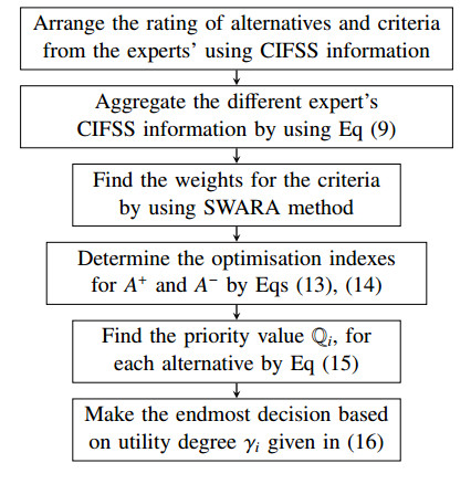
In this manuscript, we propose an integrated framework based on COmplex PRoportional ASsessment and Step-wise Weight Assessment Ratio Analysis approach within the complex intuitionistic fuzzy soft (CIFS) context. This context is an ideal technique with complex fuzzy foundation that means to denote multi-dimensional data in a concise. In this framework, criteria weights are evaluated by the SWARA technique, and the ranking of alternatives is determined by the COPRAS method using CIFSs. Further, to illustrate the applicability of the presented technique, an empirical case study of ERP software selection problem is taken. A comparative study and sensitivity analysis is presented to verify the strength of the presented methodology.

References

[1]	A. U. M. Alkouri, A. R. Salleh, Complex Intuitionistic Fuzzy Sets, AIP Conf. Proc., 1482 (2012), 464–470.
[2]	K. T. Atanassov, Intuitionistic fuzzy sets, Fuzzy Sets Syst., 20 (1986), 87–96. https://doi.org/10.1016/S0165-0114(86)80034-3 doi: 10.1016/S0165-0114(86)80034-3
[3]	J. J. Buckley, Fuzzy complex numbers, Fuzzy Sets Syst., 33 (1989), 333–345. https://doi.org/10.1016/0165-0114(89)90122-X doi: 10.1016/0165-0114(89)90122-X
[4]	D. E. Ighravwe, S. A. Oke, An integrated approach of SWARA and fuzzy COPRAS for maintenance technicians' selection factors ranking, Int. J. Syst. Assur. Eng. Manage., 10 (2019), 1615–1626. https://doi.org/10.1007/s13198-019-00912-8 doi: 10.1007/s13198-019-00912-8
[5]	F. Feng, Z. Wan, J. C. R. Alcantud, H. Garg, Three-way decision based on canonical soft sets of hesitant fuzzy sets, AIMS Math., 7 (2022), 2061–2083. https://doi.org/10.3934/math.2022118 doi: 10.3934/math.2022118
[6]	H. Garg, D. Rani, Some Generalized Complex Intuitionistic Fuzzy Aggregation Operators and Their Application to Multicriteria Decision-Making Process, Arabian J. Sci. Eng., 44 (2019), 2679–2698. https://doi.org/10.1007/s13369-018-3413-x doi: 10.1007/s13369-018-3413-x
[7]	H. Garg, R. Arora, Algorithms Based on COPRAS and Aggregation Operators with New Information Measures for Possibility Intuitionistic Fuzzy Soft Decision-Making, Math. Probl. Eng., 2020 (2020), 1563768. https://doi.org/10.1155/2020/1563768 doi: 10.1155/2020/1563768
[8]	H. Garg, Nancy, Algorithms for possibility linguistic single-valued neutrosophic decision-making based on COPRAS and aggregation operators with new information measures, Measurement, 138 (2019), 278–290. https://doi.org/10.1016/j.measurement.2019.02.031 doi: 10.1016/j.measurement.2019.02.031
[9]	H. Garg, D. Rani, New prioritized aggregation operators with priority degrees among priority orders for complex intuitionistic fuzzy information, J. Ambient Intell. Humanized Comput., 2021 (2021), 1–27. https://doi.org/10.1007/s12652-021-03164-2 doi: 10.1007/s12652-021-03164-2
[10]	M. Keil, A. Tiwana, Relative Importance of Evaluation Criteria for Enterprise Systems: A Conjoint Study, Inf. Syst. J., 16 (2006), 237–262. https://doi.org/10.1111/j.1365-2575.2006.00218.x doi: 10.1111/j.1365-2575.2006.00218.x
[11]	V. Kersuliene, E. Zavadskas, Z. Turskis, Selection of rational dispute resolution method by applying new step-wise weight assessment ratio analysis (SWARA), J. Bus. Econ. Manage., 11 (2010), 243–258. https://doi.org/10.3846/jbem.2010.12 doi: 10.3846/jbem.2010.12
[12]	Z. Kong, J. Zhao, L. Wang, J. Zhang, A new data filling approach based on probability analysis in incomplete soft sets, Expert Syst. Appl., 184 (2021), 115358. https://doi.org/10.1016/j.eswa.2021.115358 doi: 10.1016/j.eswa.2021.115358
[13]	T. Kumar, R. K. Bajaj, On complex intuitionistic fuzzy soft sets with distance measures and entropies, J. Math., 2014 (2014), 972198. https://doi.org/10.1155/2014/972198 doi: 10.1155/2014/972198
[14]	R. Kumari, A. R. Mishra, Multi-criteria COPRAS Method Based on Parametric Measures for Intuitionistic Fuzzy Sets: Application of Green Supplier Selection, Iran. J. Sci. Technol., Trans. Electr. Eng., 44 (2020), 1645–1662. https://doi.org/10.1007/s40998-020-00312-w doi: 10.1007/s40998-020-00312-w
[15]	J. Liu, L. Huaxiong, H. Bing, L. Yu, L. Dun, Convex combination-based consensus analysis for intuitionistic fuzzy three-way group decision, Inf. Sci., 574 (2021), 542–566. https://doi.org/10.1016/j.ins.2021.06.018 doi: 10.1016/j.ins.2021.06.018
[16]	J. Ma, L. Feng, J. Yang, Using complex fuzzy sets for strategic cost evaluation in supply chain downstream, 2017 IEEE International Conference on Fuzzy Systems (FUZZ-IEEE), 2017, 1–6. https://doi.org/10.1109/FUZZ-IEEE.2017.8015452
[17]	X. Ma, J. Zhan, M. Khan, Complex fuzzy sets with applications in signals, Comput. Appl. Math., 38 (2019), 150. https://doi.org/10.1007/s40314-019-0925-2 doi: 10.1007/s40314-019-0925-2
[18]	P. K. Maji, R. Biswas, A. R. Roy, Intuitionistic fuzzy soft sets, J. Fuzzy Math., 9 (2001), 677–692.
[19]	T. Mahmood, Z. Ali, Prioritized Muirhead mean aggregation operators under the complex single-valued neutrosophic settings and their application in multi-attribute decision making, J. Comput. Cognit. Eng., (2021). https://doi.org/10.47852/bonviewJCCE2022010104 doi: 10.47852/bonviewJCCE2022010104
[20]	A. R. Mishra, R. K. Singh, D. Motwani, Multi-criteria assessment of cellular mobile telephone service providers using intuitionistic fuzzy WASPAS method with similarity measures, Granular Comput., 4 (2019), 511–529. https://doi.org/10.1007/s41066-018-0114-5 doi: 10.1007/s41066-018-0114-5
[21]	A. R. Mishra, P. Rani, K. Pandey, A. Mardani, J. Streimikis, D. Streimikiene, et al., Novel Multi-Criteria Intuitionistic Fuzzy SWARA-COPRAS Approach for Sustainability Evaluation of the Bioenergy Production Process, Sustainability, 12 (2020), 4155. https://doi.org/10.3390/su12104155 doi: 10.3390/su12104155
[22]	A. R. Mishra, P. Rani, A. Mardani, K. R. Pardasani, K. Govindan, M. Alrasheedi, Healthcare evaluation in hazardous waste recycling using novel interval-valued intuitionistic fuzzy information based on complex proportional assessment method, Comput. Ind. Eng., 139 (2020), 106140. https://doi.org/10.1016/j.cie.2019.106140 doi: 10.1016/j.cie.2019.106140
[23]	D. Molodtsov, Soft set theory - First result, Comput. Math. Appl., 37 (1999), 19–31. https://doi.org/10.1016/S0898-1221(99)00056-5 doi: 10.1016/S0898-1221(99)00056-5
[24]	R. T. Ngan, L. H. Son, M. Ali, D. E. Tamir, N. D. Rishe, A. Kandel, Representing complex intuitionistic fuzzy set by quaternion numbers and applications to decision making, Appl. Soft Comput., 87 (2020). https://doi.org/10.1016/j.asoc.2019.105961 doi: 10.1016/j.asoc.2019.105961
[25]	S. Rajareega, J. Vimala, Operations on complex intuitionistic fuzzy soft lattice ordered group and CIFS-COPRAS method for equipment selection process, J. Intell. Fuzzy Syst., 41 (2021), 5709–5718. https://doi.org/10.3233/JIFS-189890 doi: 10.3233/JIFS-189890
[26]	S. Rajareega, J. Vimala, D. Preethi, Complex Intuitionistic Fuzzy Soft Lattice Ordered Group and Its Weighted Distance Measures, Mathematics, 8 (2020), 705. https://doi.org/10.3390/math8050705 doi: 10.3390/math8050705
[27]	S. Rajareega, J. Vimala, D. Preethi, The Role of $(\alpha, \beta)$ - Level set on Complex Intuitionistic Fuzzy Soft Lattice Ordered Groups, Int. J. Adv. Sci. Technol., 28 (2019), 116–123.
[28]	D. Ramot, R. Milo, M. Friedman, A. Kandel, Complex fuzzy sets, IEEE Trans. Fuzzy Syst., 10 (2002), 171–186. https://doi.org/10.1109/91.995119 doi: 10.1109/91.995119
[29]	D. Rani, H. Garg, Complex intuitionistic fuzzy power aggregation operators and their applications in multi-criteria decision-making, Expert Syst., 35 (2018), e12325. https://doi.org/10.1111/exsy.12325 doi: 10.1111/exsy.12325
[30]	P. Rani, A. R. Mishra, R. Krishankumar, A. Mardani, F. Cavallaro, K. S. Ravichandran, et al., Hesitant Fuzzy SWARA-Complex Proportional Assessment Approach for Sustainable Supplier Selection (HF-SWARA-COPRAS), Symmetry, 12 (2020), 1152. https://doi.org/10.3390/sym12071152 doi: 10.3390/sym12071152
[31]	M. Unver, M. Olgun, E. Turkarslan, Cosine and cotangent similarity measures based on Choquet integral for Spherical fuzzy sets and applications to pattern recognition, J. Comput. Cognit. Eng., (2021). https://doi.org/10.47852/bonviewJCCE2022010105 doi: 10.47852/bonviewJCCE2022010105
[32]	F. Xiao, CEQD: A complex mass function to predict interference effects, IEEE Trans. Cybern., 2021 (2021), 1–13. https://doi.org/10.1109/TCYB.2020.3040770 doi: 10.1109/TCYB.2020.3040770
[33]	F. Xiao, GIQ: A generalized intelligent quality-based approach for fusing multi-source information, IEEE Trans. Fuzzy Syst., 29 (2021), 2018–2031. https://doi.org/10.1109/TFUZZ.2020.2991296 doi: 10.1109/TFUZZ.2020.2991296
[34]	F. Xiao, Generalization of Dempster - Shafer theory: A complex mass function, Appl. Intell., 50 (2020), 3266–3275. https://doi.org/10.1007/s10489-019-01617-y doi: 10.1007/s10489-019-01617-y
[35]	F. Xiao, Generalized belief function in complex evidence theory, J. Intell. Fuzzy Syst., 38 (2020), 3665–3673. https://doi.org/10.3233/JIFS-179589 doi: 10.3233/JIFS-179589
[36]	J. Yang, Y. Yiyu, A three-way decision based construction of shadowed sets from Atanassov intuitionistic fuzzy sets, Inf. Sci., 577 (2021), 1–21. https://doi.org/10.1016/j.ins.2021.06.065 doi: 10.1016/j.ins.2021.06.065
[37]	J. Yang, Y. Yiyu, Z. Xianyong, A model of three-way approximation of intuitionistic fuzzy sets, Int. J. Mach. Learn. Cybern., 2021 (2021), 1–12. https://doi.org/10.1007/s13042-021-01380-y doi: 10.1007/s13042-021-01380-y
[38]	L. A. Zadeh, Fuzzy sets, Inf. Control, 8 (1965), 338–353. https://doi.org/10.1016/S0019-9958(65)90241-X doi: 10.1016/S0019-9958(65)90241-X
[39]	E. Zavadskas, A. Kaklauskas, V. Sarka, The new method of multi criteria complex proportional assessment of projects, Technol. Econ. Dev. Econ., 1 (1994), 131–139.

Reader Comments

Your name:*

Email:*
© 2022 the Author(s), licensee AIMS Press. This is an open access article distributed under the terms of the Creative Commons Attribution License (http://creativecommons.org/licenses/by/4.0)