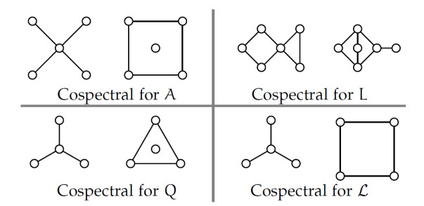
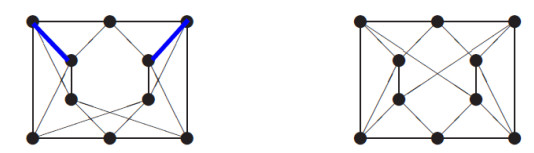
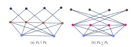
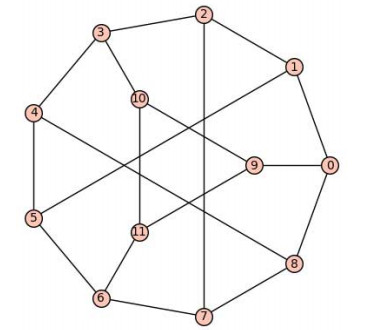
This paper delves into three research directions, leveraging the Lovász $ \vartheta $-function of a graph. First, it focuses on the Shannon capacity of graphs, providing new results that determine the capacity for two infinite subclasses of strongly regular graphs, and extending prior results. The second part explores cospectral and nonisomorphic graphs, drawing on a work by Berman and Hamud (2024), and it derives related properties of two types of joins of graphs. For every even integer such that $ n \geq 14 $, it is constructively proven that there exist connected, irregular, cospectral, and nonisomorphic graphs on $ n $ vertices, being jointly cospectral with respect to their adjacency, Laplacian, signless Laplacian, and normalized Laplacian matrices, while also sharing identical independence, clique, and chromatic numbers, but being distinguished by their Lovász $ \vartheta $-functions. The third part focuses on establishing bounds on graph invariants, particularly emphasizing strongly regular graphs and triangle-free graphs, and compares the tightness of these bounds to existing ones. The paper derives spectral upper and lower bounds on the vector and strict vector chromatic numbers of regular graphs, providing sufficient conditions for the attainability of these bounds. Exact closed-form expressions for the vector and strict vector chromatic numbers are derived for all strongly regular graphs and for all graphs that are vertex- and edge-transitive, demonstrating that these two types of chromatic numbers coincide for every such graph. This work resolves a query regarding the variant of the $ \vartheta $-function by Schrijver and the identical function by McEliece et al. (1978). It shows, by a counterexample, that the $ \vartheta $-function variant by Schrijver does not possess the property of the Lovász $ \vartheta $-function of forming an upper bound on the Shannon capacity of a graph. This research paper also serves as a tutorial of mutual interest in zero-error information theory and algebraic graph theory.
Citation: Igal Sason. Observations on graph invariants with the Lovász $ \vartheta $-function[J]. AIMS Mathematics, 2024, 9(6): 15385-15468. doi: 10.3934/math.2024747
This paper delves into three research directions, leveraging the Lovász $ \vartheta $-function of a graph. First, it focuses on the Shannon capacity of graphs, providing new results that determine the capacity for two infinite subclasses of strongly regular graphs, and extending prior results. The second part explores cospectral and nonisomorphic graphs, drawing on a work by Berman and Hamud (2024), and it derives related properties of two types of joins of graphs. For every even integer such that $ n \geq 14 $, it is constructively proven that there exist connected, irregular, cospectral, and nonisomorphic graphs on $ n $ vertices, being jointly cospectral with respect to their adjacency, Laplacian, signless Laplacian, and normalized Laplacian matrices, while also sharing identical independence, clique, and chromatic numbers, but being distinguished by their Lovász $ \vartheta $-functions. The third part focuses on establishing bounds on graph invariants, particularly emphasizing strongly regular graphs and triangle-free graphs, and compares the tightness of these bounds to existing ones. The paper derives spectral upper and lower bounds on the vector and strict vector chromatic numbers of regular graphs, providing sufficient conditions for the attainability of these bounds. Exact closed-form expressions for the vector and strict vector chromatic numbers are derived for all strongly regular graphs and for all graphs that are vertex- and edge-transitive, demonstrating that these two types of chromatic numbers coincide for every such graph. This work resolves a query regarding the variant of the $ \vartheta $-function by Schrijver and the identical function by McEliece et al. (1978). It shows, by a counterexample, that the $ \vartheta $-function variant by Schrijver does not possess the property of the Lovász $ \vartheta $-function of forming an upper bound on the Shannon capacity of a graph. This research paper also serves as a tutorial of mutual interest in zero-error information theory and algebraic graph theory.

| [1] |
C. E. Shannon, The zero error capacity of a noisy channel, IEEE T. Inform. Theory, 2 (1956), 8–19. https://doi.org/10.1109/TIT.1956.1056798 doi: 10.1109/TIT.1956.1056798

|
| [2] | N. Alon, Graph powers, In: Contemporary Combinatorics (B. Bollobás, Ed.), Bolyai Soc. Math. Stud., Springer, Budapest, Hungary, 10 (2002), 11–28. Available from: https://www.tau.ac.il/nogaa/PDFS/cap2.pdf. |
| [3] | N. Alon, Lovász, vectors, graphs and codes, In: Building Bridges Ⅱ—Mathematics of László Lovász (I. Bárány, G. O. H. Katona and A. Sali, Eds.), Bolyai Soc. Math. Stud., Springer, Budapest, Hungary, 28 (2019), 1–16. https://doi.org/10.1007/978-3-662-59204-5_1 |
| [4] | M. Jurkiewicz, A survey on known values and bounds on the Shannon capacity, In: {Selected Topics in Modern Mathematics - Edition 2014}, eds. G. Gancarzewicz, M. Skrzyński, Publishing House AKAPIT, Kraków, Poland, 2014,115–128. Available from: https://repozytorium.biblos.pk.edu.pl/resources/25729. |
| [5] |
J. Körner, A. Orlitsky, Zero-error information theory, IEEE T. Inform. Theory, 44 (1998), 2207–2229. https://doi.org/10.1109/18.720537 doi: 10.1109/18.720537
|
| [6] |
N. Alon, The Shannon capacity of a union, Combinatorica, 18 (1998), 301–310. https://doi.org/10.1007/PL00009824 doi: 10.1007/PL00009824
|
| [7] |
F. Guo, Y. Watanabe, On graphs in which the Shannon capacity is unachievable by finite product, IEEE T. Inform. Theory, 36 (1990), 622–623. https://doi.org/10.1109/18.54907 doi: 10.1109/18.54907
|
| [8] |
N. Alon, E. Lubetzky, The Shannon capacity of a graph and the independence numbers of its powers, IEEE T. Inform. Theory, 52 (2006), 2172–2176. https://doi.org/10.1109/TIT.2006.872856 doi: 10.1109/TIT.2006.872856
|
| [9] | H. Boche, C. Deppe, Computability of the zero-error capacity with Kolmogorov oracle, In: Proc. 2020 IEEE Int. Symp. Inform. Theory, Los Angeles, CA, USA, 2020, 2038–2043. https://doi.org/10.1109/ISIT44484.2020.9173984 |
| [10] | H. Boche, C. Deppe, Computability of the zero-error capacity of noisy channels, In: Proc. 2021 IEEE Inform. Theory Workshop, Kanazawa, Japan, 2021, 1–6. https://doi.org/10.1109/ITW48936.2021.9611383 |
| [11] |
L. Lovász, On the Shannon capacity of a graph, IEEE T. Inform. Theory, 25 (1979), 1–7. https://doi.org/10.1109/TIT.1979.1055985 doi: 10.1109/TIT.1979.1055985
|
| [12] |
D. E. Knuth, The sandwich theorem, Electron. J. Combin., 1 (1994), 1–48. https://doi.org/10.37236/1193 doi: 10.37236/1193
|
| [13] |
W. H. Haemers, On some problems of Lovász concerning the Shannon capacity of a graph, IEEE T. Inform. Theory, 25 (1979), 231–232. https://doi.org/10.1109/TIT.1979.1056027 doi: 10.1109/TIT.1979.1056027
|
| [14] |
B. Bukh, C. Cox, On a fractional version of Haemers' bound, IEEE T. Inform. Theory, 65 (2019), 3340–3348. https://doi.org/10.1109/TIT.2018.2889108 doi: 10.1109/TIT.2018.2889108
|
| [15] |
S. Hu, I. Tamo, O. Sheyevitz, A bound on the Shannon capacity via a linear programming variation, SIAM J. Discrete Math., 32 (2018), 2229–2241. https://doi.org/10.1137/17M115565X doi: 10.1137/17M115565X
|
| [16] |
Y. Bi, A. Tang, On upper bounding Shannon capacity of graph through generalized conic programming, Optim. Lett., 13 (2019), 1313–1323. https://doi.org/10.1007/s11590-019-01436-7 doi: 10.1007/s11590-019-01436-7
|
| [17] | V. Guruswami, A. Riazanov, Linear Shannon capacity of Cayley graphs, In: Proc. 2021 IEEE Int. Symp. Inform. Theory, Melbourne, Australia, 2021,988–992. https://doi.org/10.1109/ISIT45174.2021.9517713 |
| [18] | S. Alipour, A. Gohari, Relative fractional independence number and its applications, arXiv preprint, 2023. https://doi.org/10.48550/arXiv.2307.06155 |
| [19] |
J. Zuiddam, The asymptotic spectrum of graphs and the Shannon capacity, Combinatorica, 39 (2019), 1173–1184. https://doi.org/10.1007/s00493-019-3992-5 doi: 10.1007/s00493-019-3992-5
|
| [20] |
V. Strassen, The asymptotic spectrum of tensors, J. Reine Angew. Math., 384 (1988), 102–152. https://doi.org/10.1515/crll.1988.384.102 doi: 10.1515/crll.1988.384.102
|
| [21] | A. Wigderson, J. Zuiddam, Asymptotic spectra: Theory, applications and extensions, preprint, 2023. Available from: https://staff.fnwi.uva.nl/j.zuiddam/papers/convexity.pdf. |
| [22] |
I. Balla, O. Janzer, B. Sudakov, On MaxCut and the Lovász theta function, Proc. Amer. Math. Soc., 152 (2024), 1871–1879. https://doi.org/10.1090/proc/16675 doi: 10.1090/proc/16675
|
| [23] |
M. Dalai, Lower bounds on the probability of error for classical and classical-quantum channels, IEEE T. Inform. Theory, 59 (2013), 8027–8056. https://doi.org/10.1109/TIT.2013.2283794 doi: 10.1109/TIT.2013.2283794
|
| [24] | M. Dalai, Lovász's theta function, Rényi's divergence and the sphere-packing bound, In: Proc. 2013 IEEE Int. Symp. Inform. Theory, Istanbul, Turkey, 2013, 2038–2043. https://doi.org/10.1109/ISIT.2013.6620222 |
| [25] |
R. Duan, S. Severini, A. Winter, Zero-error communication via quantum channels, noncommutative graphs, and a quantum Lovász number, IEEE T. Inform. Theory, 59 (2013), 1164–1174. https://doi.org/10.1109/TIT.2012.2221677 doi: 10.1109/TIT.2012.2221677
|
| [26] |
G. Boreland, I. G. Todorov, A. Winter, Sandwich theorems and capacity bounds for non-commutative graphs, J. Combin. Theory Ser. A, 177 (2021), 105302. https://doi.org/10.1016/j.jcta.2020.105302 doi: 10.1016/j.jcta.2020.105302
|
| [27] |
M. Grötschel, L. Lovász, A. Schrijver, The ellipsoid method and its consequences in combinatorial optimization, Combinatorica, 1 (1981), 168–197. https://doi.org/10.1007/BF02579273 doi: 10.1007/BF02579273
|
| [28] |
M. Grötschel, L. Lovász, A. Schrijver, Polynomial algorithms for perfect graphs, Ann. Discrete Math., 21 (1984), 325–356. https://doi.org/10.1016/S0304-0208(08)72943-8 doi: 10.1016/S0304-0208(08)72943-8
|
| [29] |
L. Lovász, Graphs and geometry, American Mathematical Society, 65 (2019). https://doi.org/10.1090/coll/065 doi: 10.1090/coll/065
|
| [30] | M. R. Garey, D. S. Johnson, Computers and intractability: A guide to the theory of NP-completeness, W. H. Freeman and Company, 1979. https://doi.org/10.1137/1024022 |
| [31] |
E. R. van Dam, W. H. Haemers, Which graphs are determined by their spectrum? Linear Algebra Appl., 343 (2003), 241–272. https://doi.org/10.1016/S0024-3795(03)00483-X doi: 10.1016/S0024-3795(03)00483-X
|
| [32] |
S. Hamud, A. Berman, New constructions of nonregular cospectral graphs, Spec. Matrices, 12 (2024), 1–21. https://doi.org/10.1515/spma-2023-0109 doi: 10.1515/spma-2023-0109
|
| [33] | S. Hamud, Contributions to spectral graph theory, Ph.D. dissertation, Technion-Israel Institute of Technology, Haifa, Israel, 2023. |
| [34] |
I. Sason, Observations on Lovász $\vartheta$-function, graph capacity, eigenvalues, and strong products, Entropy, 25 (2023), 104, 1–40. https://doi.org/10.3390/e25010104 doi: 10.3390/e25010104
|
| [35] |
N. Alon, Explicit Ramsey graphs and orthonormal labelings, Electron. J. Combin., 1 (1994), 1–8. https://doi.org/10.37236/1192 doi: 10.37236/1192
|
| [36] | R. J. McEliece, E. R. Rodemich, H. C. Rumsey, The Lovász bound and some generalizations, J. Combin. Inform. Syst. Sci., 3 (1978), 134–152. Available from: https://ipnpr.jpl.nasa.gov/progress_report2/42-45/45I.PDF. |
| [37] |
A. Schrijver, A comparison of the Delsarte and Lovász bounds, IEEE T. Inform. Theory, 25 (1979), 425–429. https://doi.org/10.1109/TIT.1979.1056072 doi: 10.1109/TIT.1979.1056072
|
| [38] | E. R. Scheinerman, D. H. Ullman, Fractional graph theory: A rational approach to the theory of graphs, Dover Publications, 2013. Available from: https://www.ams.jhu.edu/ers/wp-content/uploads/2015/12/fgt.pdf. |
| [39] |
L. Lovász, On the ratio of optimal integral and fractional covers, Discrete Math., 13 (1975), 383–390. https://doi.org/10.1016/0012-365X(75)90058-8 doi: 10.1016/0012-365X(75)90058-8
|
| [40] |
J. W. Moon, L. Moser, On cliques in graphs, Isr. J. Math., 3 (1965), 23–28. https://doi.org/10.1007/BF02760024 doi: 10.1007/BF02760024
|
| [41] | A. E. Brouwer, W. H. Haemers, Spectra of graphs, Springer, New York, NY, USA, 2012. https://doi.org/10.1007/978-1-4614-1939-6 |
| [42] | G. Chartrand, L. Lesniak, P. Zhang, Graphs and digraphs, 6 Eds., CRC Press, 2015. https://doi.org/10.1201/b19731 |
| [43] | S. M. Cioabǎ, M. R. Murty, A first course in graph theory and combinatorics, 2 Eds., Springer, 2022. https://doi.org/10.1007/978-981-19-0957-3 |
| [44] | D. Cvetković, P. Rowlinson, S. Simić, An introduction to the theory of graph spectra, London Mathematical Society Student Texts 75, Cambridge University Press, 2009. https://doi.org/10.1017/CBO9780511801518 |
| [45] | C. Godsil, G. Royle, Algebraic graph theory, Springer, 2001. https://doi.org/10.1007/978-1-4613-0163-9 |
| [46] | B. Nica, A brief introduction to spectral graph theory, European Mathematical Society, 2018. https://doi.org/10.4171/188 |
| [47] | Z. Stanić, Inequalities for graph eigenvalues, London Mathematical Society Lecture Note Series, Series Number 423, Cambridge University Press, 2015. https://doi.org/10.1017/CBO9781316341308 |
| [48] |
L. Liu, B. Ning, Unsolved problems in spectral graph theory, Oper. Res. Trans., 27 (2023), 34–60. https://doi.org/10.15960/j.cnki.issn.1007-6093.2023.04.003 doi: 10.15960/j.cnki.issn.1007-6093.2023.04.003
|
| [49] | S. Butler, Algebraic aspects of the normalized Laplacian, In: Recent Trends in Combinatorics, the IMA Volumes in Mathematics and its Applications, 159 (2016), 295–315. https://doi.org/10.1007/978-3-319-24298-9_13 |
| [50] |
D. Cvetković, P. Rowlinson, S. Simić, Signless Laplacians of finite graphs, Linear Algebra Appl., 423 (2007), 155–171. https://doi.org/10.1016/j.laa.2007.01.009 doi: 10.1016/j.laa.2007.01.009
|
| [51] | The Sage Developers, SageMath, the Sage Mathematics Software System, Version 9.3, 2021. |
| [52] | A. E. Brouwer, H. Van Maldeghem, Strongly regular graphs, Cambridge University Press, Encyclopedia of Mathematics and its Applications, 18 (2022). https://doi.org/10.1017/9781009057226 |
| [53] |
X. Xu, S. P. Radziszowski, Bounds on Shannon capacity and Ramsey numbers from product of graphs, IEEE T. Inform. Theory, 59 (2013), 4767–4770. https://doi.org/10.1109/TIT.2013.2256951 doi: 10.1109/TIT.2013.2256951
|
| [54] |
T. Bohman, R. Holzman, A nontrivial lower bound on the Shannon capacities of the complements of odd cycles, IEEE T. Inform. Theory, 49 (2003), 721–722. https://doi.org/10.1109/TIT.2002.808128 doi: 10.1109/TIT.2002.808128
|
| [55] | T. Bohman, A limit theorem for the Shannon capacities of odd cycles. I, Proc. Amer. Math. Soc., 131 (2003), 3559–3569. Available from: http://www.jstor.org/stable/1194666. |
| [56] | T. Bohman, A limit theorem for the Shannon capacities of odd cycles. Ⅱ, Proc. Amer. Math. Soc., 133 (2005), 537–543. Available from: http://www.jstor.org/stable/4097960. |
| [57] |
T. Bohman, R. Holzman, V. Natarajan, Maximum independent sets in certain powers of odd cycles, Electron. J. Combin., 16 (2009), 1–8. https://doi.org/10.37236/264 doi: 10.37236/264
|
| [58] |
T. Bohman, R. Holzman, V. Natarajan, On the independence numbers of the cubes of odd cycles, Electron. J. Combin., 20 (2013), 1–19. https://doi.org/10.37236/2598 doi: 10.37236/2598
|
| [59] |
R. S. Hales, Numerical invariants and the strong product of graphs, J. Combin. Theory Ser. B, 15 (1973), 146–155. https://doi.org/10.1016/0095-8956(73)90014-2 doi: 10.1016/0095-8956(73)90014-2
|
| [60] |
S. C. Polak, A. Schrijver, New lower bound on the Shannon capacity of $ \mathsf{C}_{{7}}$ from circular graphs, Inform. Process. Lett., 143 (2019), 37–40. https://doi.org/10.1016/j.ipl.2018.11.006 doi: 10.1016/j.ipl.2018.11.006
|
| [61] |
E. Sonnemann, O. Krafft, Independence numbers of product graphs, J. Combin. Theory Ser. B, 17 (1974), 133–142. https://doi.org/10.1016/0095-8956(74)90081-1 doi: 10.1016/0095-8956(74)90081-1
|
| [62] | D. G. Zhu, An improved lower bound on the Shannon capacities of complements of odd cycles, arXiv preprint, 2024. https://doi.org/10.48550/arXiv.2402.10025 |
| [63] |
P. Hell, F. S. Roberts, Analogues of the Shannon capacity of a graph, Ann. Discrete Math., 12 (1982), 155–168. https://doi.org/10.1016/S0304-0208(08)73501-1 doi: 10.1016/S0304-0208(08)73501-1
|
| [64] |
P. Keevash, E. Long, On the normalized Shannon capacity of a union, Combin. Probab. Comput., 25 (2016), 766–767. https://doi.org/10.1017/S0963548316000055 doi: 10.1017/S0963548316000055
|
| [65] |
A. Schrijver, On the Shannon capacity of sums and products of graphs, Indag. Math., 34 (2023), 37–41. https://doi.org/10.1016/j.indag.2022.08.009 doi: 10.1016/j.indag.2022.08.009
|
| [66] |
G. Simonyi, Shannon capacity and the categorical product, Electron. J. Combin., 28 (2021), 1–23. https://doi.org/10.37236/9113 doi: 10.37236/9113
|
| [67] |
L. Lovász, M. Saks, A. Schrijver, Orthogonal representations and connectivity of graphs, Linear Algebra Appl., 114–115 (1989), 439–454. https://doi.org/10.1016/0024-3795(89)90475-8 doi: 10.1016/0024-3795(89)90475-8
|
| [68] | I. Balla, Orthonormal representations, vector chromatic number, and extension complexity, arXiv preprint, 2023. https://doi.org/10.48550/arXiv.2310.17482 |
| [69] |
I. Balla, S. Letzter, B. Sudakov, Orthonormal representations of $\mathsf{{H}}$-free graphs, Discrete Comput. Geom., 64 (2020), 654–670. https://doi.org/10.1007/s00454-020-00185-0 doi: 10.1007/s00454-020-00185-0
|
| [70] |
D. Karger, M. Motwani, M. Sudan, Approximate graph coloring by semidefinite programming, J. ACM, 45 (1998), 246–265. https://doi.org/10.1145/274787.274791 doi: 10.1145/274787.274791
|
| [71] | M. Szegedy, A note on the $\vartheta$ number of Lovász and the generalized Delsarte bound, In: Proceedings of the 35th Annual Symposium on Foundations of Computer Science, Santa Fe, New Mexico, USA, 1994, 36–39. https://doi.org/10.1109/SFCS.1994.365707 |
| [72] |
Y. Bilu, Tales of Hoffman: Three extensions of Hoffman's bound on the graph chromatic number, J. Combin. Theory Ser. B, 96 (2006), 608–613. https://doi.org/10.1016/j.jctb.2005.10.002 doi: 10.1016/j.jctb.2005.10.002
|
| [73] |
A. Galtman, Spectral characterizations of the Lovász number and the Delsarte number of a graph, J. Algebraic Combin., 12 (2000), 131–143. https://doi.org/10.1023/A:1026587926110 doi: 10.1023/A:1026587926110
|
| [74] |
C. Godsil, D. E. Roberson, B. Rooney, R. Šámal, A. Varvitsiotis, Vector coloring the categorical product of graphs, Math. Program. Ser. A, 182 (2020), 275–314. https://doi.org/10.1007/s10107-019-01393-0 doi: 10.1007/s10107-019-01393-0
|
| [75] |
P. Wocjan, C. Elphick, D. Anekstein, More tales of Hoffman: Bounds for the vector chromatic number of a graph, Discuss. Math. Graph Theory, 43 (2023), 159–169. https://doi.org/10.7151/dmgt.2358 doi: 10.7151/dmgt.2358
|
| [76] |
A. Acín, R. Duanc, D. E. Roberson, A. B. Sainz, A. Winter, A new property of the Lovász number and duality relations between graph parameters, Discrete Appl. Math., 216 (2017), 489–501. https://doi.org/10.1016/j.dam.2016.04.028 doi: 10.1016/j.dam.2016.04.028
|
| [77] |
N. Alon, N. Kahale, Approximating the independence number via the $\vartheta$-function, Math. Program., 80 (1998), 253–264. https://doi.org/10.1007/BF01581168 doi: 10.1007/BF01581168
|
| [78] | B. Csonka, G. Simonyi, Shannon capacity, Lovász theta number, and the Mycielski construction, arXiv preprint, 2023. https://doi.org/10.48550/arXiv.2312.09224 |
| [79] |
U. Feige, Randomized graph products, chromatic numbers, and the Lovász $\vartheta$-function, Combinatorica, 17 (1997), 79–90. https://doi.org/10.1007/BF01196133 doi: 10.1007/BF01196133
|
| [80] | O. Gritsenko, On strongly regular graph with parameters $(65, 32, 15, 16)$, arXiv preprint, 2021. https://doi.org/10.48550/arXiv.2102.05432 |
| [81] |
A. Neumaier, Cliques and claws in edge-transitive strongly regular graphs, Math. Z., 174 (1980), 197–202. https://doi.org/10.1007/BF01161408 doi: 10.1007/BF01161408
|
| [82] | A. Farrugia, Self-complementary graphs and generalisations: A comprehensive reference manual, Master thesis, University of Malta, Republic of Malta, August 1999, last updated in 2003. Available from: https://alastairfarrugia.net/sc-graph.html. |
| [83] | F. Harary, Graph theory, Addison-Wesley, 1969, Reading, MA, USA. |
| [84] |
R. Mathon, On self-complementary strongly regular graphs, Discrete Math., 69 (1988), 263–281. https://doi.org/10.1016/0012-365X(88)90055-6 doi: 10.1016/0012-365X(88)90055-6
|
| [85] |
M. Muzychuk, On Sylow subgraphs of vertex-transitive self-complementary graphs, Bull. London Math. Soc., 31 (1999), 531–533. https://doi.org/10.1112/S0024609399005925 doi: 10.1112/S0024609399005925
|
| [86] |
W. Peisert, All self-complementary symmetric graphs, J. Algebra, 240 (2001), 209–229. https://doi.org/10.1006/jabr.2000.8714 doi: 10.1006/jabr.2000.8714
|
| [87] |
S. B. Rao, On regular and strongly-regular self-complementary graphs, Discrete Math., 54 (1985), 73–82. https://doi.org/10.1016/0012-365X(85)90063-9 doi: 10.1016/0012-365X(85)90063-9
|
| [88] |
I. G. Rosenberg, Regular and strongly regular self-complementary graphs, North-Holland Math. Stud., 60 (1982), 223–238. https://doi.org/10.1016/S0304-0208(08)73507-2 doi: 10.1016/S0304-0208(08)73507-2
|
| [89] |
S. Ruiz, On strongly regular self-complementary graphs, J. Graph Theory, 5 (1981), 213–215. https://doi.org/10.1002/jgt.3190050213 doi: 10.1002/jgt.3190050213
|
| [90] |
A. Sali, G. Simonyi, Orientations of self-complementary graphs and the relation of the Sperner and Shannon capacities, Eur. J. Combin., 20 (1999), 93–99. https://doi.org/10.1006/eujc.1998.0256 doi: 10.1006/eujc.1998.0256
|
| [91] | B. Zelinka, Self-complementary vertex-transitive undirected graphs, Math. Slovaca, 29 (1979), 91–95. Available from: https://eudml.org/doc/34053. |
| [92] | M. Aigner, G. M. Ziegler, Proofs from the book, 6 Eds., Springer, Berlin, Germany, 2018. Available from: https://link.springer.com/book/10.1007/978-3-662-57265-8 |
| [93] |
Z. Tang, Z. Wan, Symplectic graphs and their automorphisms, Eur. J. Combin., 27 (2006), 38–50. https://doi.org/10.1016/j.ejc.2004.08.002 doi: 10.1016/j.ejc.2004.08.002
|
| [94] |
R. D. Baker, G. L. Ebert, J. Hemmeter, A. Woldar, Maximal cliques in the Paley graph of square order, J. Stat. Plan. Inference, 56 (1996), 33–38. https://doi.org/10.1016/S0378-3758(96)00006-7 doi: 10.1016/S0378-3758(96)00006-7
|
| [95] |
A. Blokhuis, On subsets of $\mathrm{GF}(q^2)$ with square differences, Indag. Math. Proc., 87 (1984), 369–372. https://doi.org/10.1016/1385-7258(84)90036-2 doi: 10.1016/1385-7258(84)90036-2
|
| [96] |
A. Abiad, W. H. Haemers, Cospectral graphs and regular orthogonal matrices of level 2, Electron. J. Combin., 19 (2012), P13, 1–16. https://doi.org/10.37236/2383 doi: 10.37236/2383
|
| [97] |
Z. L. Blázsik, J. Cummings, W. H. Haemers, Cospectral regular graphs with and without a perfect matching, Discrete Math., 338 (2015), 199–201. https://doi.org/10.1016/1385-7258(84)90036-2 doi: 10.1016/1385-7258(84)90036-2
|
| [98] |
S. Butler, J. Grout, A construction of cospectral graphs for the normalized Laplacian, Electron. J. Combin., 18 (2011), 1–20. https://doi.org/10.37236/718 doi: 10.37236/718
|
| [99] |
E. R. van Dam, W. H. Haemers, Developments on spectral characterizations of graphs, Discrete Math., 309 (2009), 576–586. https://doi.org/10.1016/j.disc.2008.08.019 doi: 10.1016/j.disc.2008.08.019
|
| [100] |
S. Dutta, Constructing nonisomorphic signless Laplacian cospectral graphs, Discrete Math., 343 (2020), 1–12. https://doi.org/10.1016/j.disc.2019.111783 doi: 10.1016/j.disc.2019.111783
|
| [101] |
S. Dutta, B. Adhikari, Construction of cospectral graphs, J. Algebraic Combin., 52 (2020), 215–235. https://doi.org/10.1007/s10801-019-00900-y doi: 10.1007/s10801-019-00900-y
|
| [102] |
C. D. Godsil, B. D. McKay, Constructing cospectral graphs, Aequationes Math., 25 (1982), 257–268. https://doi.org/10.1007/BF02189621 doi: 10.1007/BF02189621
|
| [103] |
W. H. Haemers, E. Spence, Enumeration of cospectral graphs, Eur. J. Combin., 25 (2004), 199–211. https://doi.org/10.1016/S0195-6698(03)00100-8 doi: 10.1016/S0195-6698(03)00100-8
|
| [104] |
Z. Lu, X. Ma, M. Zhang, Spectra of graph operations based on splitting graph, J. Appl. Anal. Comput., 13 (2023), 133–155. https://doi.org/10.11948/20210446 doi: 10.11948/20210446
|
| [105] |
A. Z. Abdian, A. Behmaram, G. H. Fath-Tabar, Graphs determined by signless Laplacian spectra, AKCE Int. J. Graphs Comb., 17 (2020), 45–50. https://doi.org/10.1016/j.akcej.2018.06.009 doi: 10.1016/j.akcej.2018.06.009
|
| [106] |
A. Berman, D. M. Chen, Z. B. Chen, W. Z. Liang, X. D. Zhang, A family of graphs that are determined by their normalized Laplacian spectra, Linear Algebra Appl., 548 (2018), 66–76. https://doi.org/10.1016/j.laa.2018.03.001 doi: 10.1016/j.laa.2018.03.001
|
| [107] |
M. Liu, H. Shan, K. C. Das, Some graphs determined by their (signless) Laplacian matrix, Linear Algebra Appl., 449 (2014), 154–165. https://doi.org/10.1016/j.laa.2014.02.027 doi: 10.1016/j.laa.2014.02.027
|
| [108] |
X. Liu, P. Lu, Signless Laplacian spectral characterization of some joins, Electron. J. Linear Algebra, 30 (2015), 443–454. https://doi.org/10.13001/1081-3810.1942 doi: 10.13001/1081-3810.1942
|
| [109] |
X. Liu, Y. Zhang, X. Gui, The multi-fan graphs are determined by their Laplacian spectra, Discrete Math., 308 (2008), 4267–4271. https://doi.org/10.1016/j.disc.2007.08.002 doi: 10.1016/j.disc.2007.08.002
|
| [110] |
G. R. Omidi, K. Tajbakhsh, Starlike trees are determined by their Laplacian spectrum, Linear Algebra Appl., 422 (2007), 654–658. https://doi.org/10.1016/j.laa.2006.11.028 doi: 10.1016/j.laa.2006.11.028
|
| [111] |
M. Laurent, A. Schrijver, On Leonid Gurvits's proof for permanents, Am. Math. Mon., 117 (2010), 903–911. https://doi.org/10.4169/000298910X523380 doi: 10.4169/000298910X523380
|
| [112] | J. H. van Lint, R. M. Wilson, A course in combinatorics, 2 Eds., Cambridge University Press, 2001. https://doi.org/10.1017/CBO9780511987045 |
| [113] | M. Grant, S. Boyd, CVX: Matlab software for disciplined convex programming, version 2.2, 2020. Available from: http://cvxr.com/cvx. |
| [114] | J. R. Alfonsín, B. A. Reed, Perfect graphs, John Wiley and Sons Publishers, 2001. |
| [115] | L. W. Beineke, M. C. Golumbic, R. J. Wilson, Topics in algorithmic graph theory, Cambridge University Press, 2021. https://doi.org/10.1017/9781108592376 |
| [116] | M. C. Golumbic, Algorithmic graph theory and perfect graphs, 2 Eds., Elsevier, 2004. |
| [117] | C. Berge, Perfect graphs, In: Six Papers on Graph Theory, Indian Statistical Institute, 1963, 1–21. |
| [118] | L. Lovász, Perfect graphs, In: Selected Topics in Graph Theory 2, eds. W. L. Beineke, R. J. Wilson, Academic Press, 1983, 55–87. |
| [119] |
L. Lovász, Normal hypergraphs and the perfect graph conjecture, Discrete Math., 2 (1972), 253–272. https://doi.org/10.1016/0012-365X(72)90006-4 doi: 10.1016/0012-365X(72)90006-4
|
| [120] |
M. Chudnovsky, N. Robertson, P. Seymour, R. Thomas, The strong perfect graph theorem, Ann. Math., 164 (2006), 51–229. https://doi.org/10.4007/annals.2006.164.51 doi: 10.4007/annals.2006.164.51
|
| [121] | N. Trotignon, Perfect graphs: A survey, In: Topics in Chromatic Graph Theory, Cambridge University Press, 2015,137–160. https://doi.org/10.1017/CBO9781139519793.010 |
| [122] |
J. Balogh, F. C. Clemen, F. Lidický, S. Norin, J. Volec, The spectrum of triangle-free graphs, SIAM J. Discrete Math., 37 (2023), 1173–1179. https://doi.org/10.1137/22M150767X doi: 10.1137/22M150767X
|
| [123] |
P. Csikvári, Note on the sum of the smallest and largest eigenvalues of a triangle-free graph, Linear Algebra Appl., 650 (2022), 92–97. https://doi.org/10.1016/j.laa.2022.06.004 doi: 10.1016/j.laa.2022.06.004
|
| [124] |
A. Berman, M. Dür, N. Shaked-Monderer, J. Witzel, Cutting planes for semidefinite relaxations based on triangle-free subgraphs, Optim. Lett., 10 (2016), 433–446. https://doi.org/10.1007/s11590-015-0922-3 doi: 10.1007/s11590-015-0922-3
|
| [125] |
A. Berman, N. Shaked-Monderer, Triangle-free graphs and completely positive matrices, Cent. Eur. J. Oper. Res., 30 (2022), 1093–1099. https://doi.org/10.1007/s10100-021-00750-9 doi: 10.1007/s10100-021-00750-9
|
| [126] |
A. Bernshteyn, T. Brazelton, R. Cao, A. Kang, Counting colorings of triangle-free graphs, J. Combin. Theory Ser. B, 161 (2023), 86–108. https://doi.org/10.1016/j.jctb.2023.02.004 doi: 10.1016/j.jctb.2023.02.004
|
| [127] |
F. Pirot, J. S. Sereni, Fractional chromatic number, maximum degree, and girth, SIAM J. Discrete Math., 35 (2021), 2815–2843. https://doi.org/10.1137/20M1382283 doi: 10.1137/20M1382283
|
| [128] |
S. Glock, O. Janzer, B. Sudakov, New results for MaxCut in H-free graphs, J. London Math. Soc., 108 (2023), 441–481. https://doi.org/10.1112/jlms.12750 doi: 10.1112/jlms.12750
|
| [129] |
P. J. Cameron, A. N. Dang, S. Riis, Guessing games on triangle-free graphs, Electron. J. Combin., 23 (2016), 1–9. https://doi.org/10.37236/4731 doi: 10.37236/4731
|
| [130] |
A. Barg, G. Zémor, High-rate storage codes on triangle-free graphs, IEEE T. Inform. Theory, 68 (2022), 7787–7797. https://doi.org/10.1109/TIT.2022.3191309 doi: 10.1109/TIT.2022.3191309
|
| [131] | A. Barg, M. Schwartz, L. Yohananov, Storage codes on coset graphs with asymptotically unit rate, arXiv preprint, 2023. https://doi.org/10.48550/arXiv.2212.12117 |
| [132] | H. Deng, H. Huang, G. Weng, Q. Xiang, The BCH family of storage codes on triangle-free graphs is of unit rate, arXiv preprint, 2023. https://doi.org/10.48550/arXiv.2310.04820 |
| [133] |
H. Huang, Q. Xiang, Construction of storage codes of rate approaching one on triangle-free graphs, Des. Codes Cryptogr., 91 (2023), 3901–3913. https://doi.org/10.1007/s10623-023-01278-6 doi: 10.1007/s10623-023-01278-6
|
| [134] |
J. B. Shearer, A note on the independence number of triangle-free graphs, Discrete Math., 46 (1983), 83–87. https://doi.org/10.1016/0012-365X(83)90273-X doi: 10.1016/0012-365X(83)90273-X
|
| [135] |
J. B. Shearer, A note on the independence number of triangle-free graphs, Ⅱ, J. Combin. Theory Ser. B, 53 (1991), 300–307. https://doi.org/10.1016/0095-8956(91)90080-4 doi: 10.1016/0095-8956(91)90080-4
|
| [136] |
J. R. Griggs, Lower bounds on the independence number in terms of the degrees, J. Combin. Theory Ser. B, 34 (1983), 22–39. https://doi.org/10.1016/0095-8956(83)90003-5 doi: 10.1016/0095-8956(83)90003-5
|
| [137] |
K. Guo, S. Spiro, New eigenvalue bound for the fractional chromatic number, J. Graph Theory, 106 (2024), 167–181. https://doi.org/10.1002/jgt.23071 doi: 10.1002/jgt.23071
|
| [138] |
A. Abiad, L. de Lima, D. N. Desai, K. Guo, L. Hogben, J. Madrid, Positive and negative square energies of graphs, Electron. J. Linear Algebra, 39 (2023), 307–326. https://doi.org/10.13001/ela.2023.7827 doi: 10.13001/ela.2023.7827
|
| [139] | C. Elphick, W. Linz, Symmetry and asymmetry between positive and negative squared energies of graphs, arXiv preprint, 2024. https://doi.org/10.48550/arXiv.2311.11530 |
| [140] |
T. Ando, M. Lin, Proof of a conjectured lower bound on the chromatic number of a graph, Linear Algebra Appl., 485 (2015), 480–484. https://doi.org/10.1016/j.laa.2015.08.007 doi: 10.1016/j.laa.2015.08.007
|
| [141] |
P. Wocjan, C. Elphick, New spectral bounds on the chromatic number encompassing all eigenvalues of the adjacency matrix, Electron. J. Combin., 20 (2013), 39. https://doi.org/10.37236/2735 doi: 10.37236/2735
|
| [142] | G. Coutinho, T. J. Spier, Sums of squares of eigenvalues and the vector chromatic number, arXiv preprint, 2023. https://doi.org/10.48550/arXiv.2308.04475 |
| [143] |
C. Elphick, P. Wocjan, An inertial lower bound for the chromatic number of a graph, Electron. J. Combin., 24 (2017), 1–9. https://doi.org/10.37236/6404 doi: 10.37236/6404
|
| [144] | V. K. Wei, A lower bound on the stability number of a simple graph, Bell Laboratories Technical Memorandum 81-11217-9, Murray Hill, New Jersey, USA, 1981. |
| [145] |
C. Edwards, C. Elphick, Lower bounds for the clique and chromatic numbers of a graph, Discrete Appl. Math., 5 (1983), 51–64. https://doi.org/10.1016/0166-218X(83)90015-X doi: 10.1016/0166-218X(83)90015-X
|
| [146] |
V. Nikiforov, Some inequalities for the largest eigenvalue of a graph, Combin. Probab. Comput., 11 (2002), 179–189. https://doi.org/10.1017/S0963548301004928 doi: 10.1017/S0963548301004928
|
| [147] |
T. Motzkin, E. Straus, Maxima for graphs and a new proof of a theorem of Turán, Can. J. Math., 17 (1965), 533–540. https://doi.org/10.4153/CJM-1965-053-6 doi: 10.4153/CJM-1965-053-6
|
| [148] |
H. S. Wilf, Spectral bounds for the clique and independence numbers of graphs, J. Combin. Theory Ser. B, 40 (1986), 113–117. https://doi.org/10.1016/0095-8956(86)90069-9 doi: 10.1016/0095-8956(86)90069-9
|
| [149] |
V. Nikiforov, More spectral bounds on the clique and independence numbers, J. Combin. Theory Ser. B, 99 (2009), 819–826. https://doi.org/10.1016/j.jctb.2009.01.003 doi: 10.1016/j.jctb.2009.01.003
|
| [150] |
M. Lu, H. Liu, F. Tian, Laplacian spectral bounds for clique and independence numbers of graphs, J. Combin. Theory Ser. B, 97 (2007), 726–732. https://doi.org/10.1016/j.jctb.2006.12.003 doi: 10.1016/j.jctb.2006.12.003
|
| [151] | W. H. Haemers, Eigenvalue techniques in design and graph theory, Ph.D. dissertation, Stichting Mathematisch Centrum, Amsterdam, Netherlands, 1979. https://doi.org/10.6100/IR41103 |
| [152] | P. Delsarte, An algebraic approach to the association schemes of coding theory, Philips Res. Rep. Suppl., 10 (1973), 1–97. |
| [153] |
W. H. Haemers, Hoffman's ratio bound, Linear Algebra Appl., 617 (2021), 215–219. https://doi.org/10.1016/j.laa.2021.02.010 doi: 10.1016/j.laa.2021.02.010
|
| [154] |
C. D. Godsil, M. W. Newman, Eigenvalue bounds for independent sets, J. Combin. Theory Ser. B, 98 (2008), 721–734. https://doi.org/10.1016/j.jctb.2007.10.007 doi: 10.1016/j.jctb.2007.10.007
|
| [155] |
Y. Li, Z. Zhang, A note on eigenvalue bounds for independence numbers of nonregular graphs, Discrete Appl. Math., 174 (2014), 146–149. https://doi.org/10.1016/j.dam.2014.04.008 doi: 10.1016/j.dam.2014.04.008
|
| [156] |
D. F. Holt, A graph which is edge transitive but not arc transitive, J. Graph Theory, 5 (1981), 201–204. https://doi.org/10.1002/jgt.3190050210 doi: 10.1002/jgt.3190050210
|
| [157] |
A. Nilli, Triangle-free graphs with large chromatic numbers, Discrete Math., 211 (2000), 261–262. https://doi.org/10.1016/S0012-365X(99)00109-0 doi: 10.1016/S0012-365X(99)00109-0
|
| [158] | S. Niskanen, P. R. J. Österg$\mathring{\mathrm{a}}$rd, Cliquer user's guide, Version 1.0, Technical Report T48, Communications Laboratory, Helsinki University of Technology, Espoo, Finland, 2003. Available from: https://users.aalto.fi/pat/cliquer/cliquer_fm.pdf. |
| [159] |
Q. Wu, J. K. Hao, A review on algorithms for maximum clique problems, Eur. J. Oper. Res., 242 (2015), 693–709. https://doi.org/10.1016/j.ejor.2014.09.064 doi: 10.1016/j.ejor.2014.09.064
|
| [160] |
F. Juhász, The asymptotic behaviour of Lovász $\vartheta$-function for random graphs, Combinatorica, 2 (1982), 153–155. https://doi.org/10.1007/BF02579314 doi: 10.1007/BF02579314
|
| [161] |
A. Coja-Oghlan, The Lovász number of random graphs, Combin. Probab. Comput., 14 (2005), 439–465. https://doi.org/10.1017/S0963548305006826 doi: 10.1017/S0963548305006826
|
Figures(6) / Tables(6)

Igal Sason. Observations on graph invariants with the Lovász $ \vartheta $-function[J]. AIMS Mathematics, 2024, 9(6): 15385-15468. doi: 10.3934/math.2024747


 DownLoad: