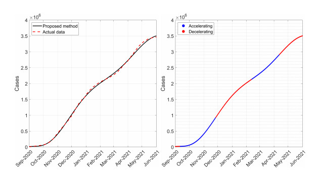
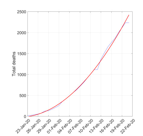
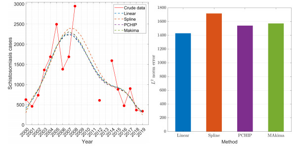
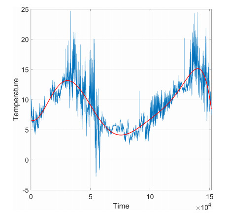
Data smoothing is a method that involves finding a sequence of values that exhibits the trend of a given set of data. This technique has useful applications in dealing with time series data with underlying fluctuations or seasonality and is commonly carried out by solving a minimization problem with a discrete solution that takes into account data fidelity and smoothness. In this paper, we propose a method to obtain the smooth approximation of data by solving a minimization problem in a function space. The existence of the unique minimizer is shown. Using polynomial basis functions, the problem is projected to a finite dimension. Unlike the standard discrete approach, the complexity of our method does not depend on the number of data points. Since the calculated smooth data is represented by a polynomial, additional information about the behavior of the data, such as rate of change, extreme values, concavity, etc., can be drawn. Furthermore, interpolation and extrapolation are straightforward. We demonstrate our proposed method in obtaining smooth mortality rates for the Philippines, analyzing the underlying trend in COVID-19 datasets, and handling incomplete and high-frequency data.
Citation: Rolly Czar Joseph Castillo, Renier Mendoza. On smoothing of data using Sobolev polynomials[J]. AIMS Mathematics, 2022, 7(10): 19202-19220. doi: 10.3934/math.20221054
Data smoothing is a method that involves finding a sequence of values that exhibits the trend of a given set of data. This technique has useful applications in dealing with time series data with underlying fluctuations or seasonality and is commonly carried out by solving a minimization problem with a discrete solution that takes into account data fidelity and smoothness. In this paper, we propose a method to obtain the smooth approximation of data by solving a minimization problem in a function space. The existence of the unique minimizer is shown. Using polynomial basis functions, the problem is projected to a finite dimension. Unlike the standard discrete approach, the complexity of our method does not depend on the number of data points. Since the calculated smooth data is represented by a polynomial, additional information about the behavior of the data, such as rate of change, extreme values, concavity, etc., can be drawn. Furthermore, interpolation and extrapolation are straightforward. We demonstrate our proposed method in obtaining smooth mortality rates for the Philippines, analyzing the underlying trend in COVID-19 datasets, and handling incomplete and high-frequency data.

| [1] | Philippine intercompany mortality study 2017, Actuarial Society of the Philippines, 2017. Available from: http://www.actuary.org.ph/wp-content/uploads/2017/05/2017-PICM-Study-Final-Report-18May2017.pdf. |
| [2] |
L. Ambrosio, V. M. Tortelli, Approximation of functional depending on jumps by elliptic functional via t-convergence, Commun. Pure Appl. Math., 43 (1990), 999–1036. https://doi.org/10.1002/cpa.3160430805 doi: 10.1002/cpa.3160430805

|
| [3] |
A. Brandenburg, Piecewise quadratic growth during the 2019 novel coronavirus epidemic, Infect. Dis. Model., 5 (2020), 681–690. https://doi.org/10.1016/j.idm.2020.08.014 doi: 10.1016/j.idm.2020.08.014
|
| [4] |
R. J. Brooks, M. Stone, F. Y. Chan, L. K. Chan, Cross-validatory graduation, Insur. Math. Econ., 7 (1988), 59–66. https://doi.org/10.1016/0167-6687(88)90097-2 doi: 10.1016/0167-6687(88)90097-2
|
| [5] | M. A. Buford, W. L. Hafley, Probability distributions as models for mortality, Forest Sci., 31 (1985), 331–341. |
| [6] |
R. H. Byrd, J. C. Gilbert, J. Nocedal, A trust region method based on interior point techniques for nonlinear programming, Math. Program., 89 (2000), 149–185. https://doi.org/10.1007/PL00011391 doi: 10.1007/PL00011391
|
| [7] |
F. Y. Chan, L. K. Chan, E. R. Mead, Properties and modifications of Whittaker-Henderson graduation, Scand. Actuar. J., 1982 (1982), 57–61. https://doi.org/10.1080/03461238.1982.10405433 doi: 10.1080/03461238.1982.10405433
|
| [8] | G. Chowell, Fitting dynamic models to epidemic outbreaks with quantified uncertainty: A primer for parameter uncertainty, identifiability, and forecasts, Infect. Dis. Model., 2 (2017), 379–398. |
| [9] | D. Cioranescu, P. Donato, M. P. Roque, An introduction to second order partial differential equations: Classical and variational solutions, World Scientific, Singapore, 2018. |
| [10] | B. Efron, R. J. Tibshirani, An introduction to the bootstrap, CRC Press, 1992. |
| [11] |
P. H. Eilers, A perfect smoother, Anal. Chemis., 75 (2003), 3631–3636. https://doi.org/10.1021/ac034173t doi: 10.1021/ac034173t
|
| [12] |
D. Garcia, Robust smoothing of gridded data in one and higher dimensions with missing values, Comput. Stat. Data Anal., 54 (2010), 1167–1178. https://doi.org/10.1016/j.csda.2009.09.020 doi: 10.1016/j.csda.2009.09.020
|
| [13] | L. Grafakos, Classical Fourier analysis, Springer, New York, 2008. |
| [14] | P. Graven, Smoothing noisy data with spline function: Estimating the correct degree of smoothing by the method of Generalized Cross-Validaton, Numer. Math., 31 (1978), 377–403. |
| [15] |
V. Guerrero, E. Silva, Smoothing a time series by segments of the data range, Commun. Stat.-Theor. M., 44 (2015), 4568–4585. https://doi.org/10.1080/03610926.2014.901372 doi: 10.1080/03610926.2014.901372
|
| [16] |
V. Guerrero, Estimating trends with percentage of smoothness chosen by the user, Int. Stat. Rev., 76 (2008), 182–202. https://doi.org/10.1111/j.1751-5823.2008.00047.x doi: 10.1111/j.1751-5823.2008.00047.x
|
| [17] | R. Hannah, E. Mathieu, L. Rodés-Guirao, C. Appel, C. Giattino, E. Ortiz-Ospina, et al., Coronavirus pandemic (COVID-19), Our World in Data, 2020. Available from: https://ourworldindata.org/coronavirus. |
| [18] | S. Hansun, A new approach of moving average method in time series analysis, 2013 conference on new media studies (CoNMedia), IEEE, 2013, 1–4. |
| [19] |
Y. He, X. Wang, H. He, J. Zhai, B. Wang, Moving average based index for judging the peak of COVID-19 epidemic, Int. J. Environ. Res. Pub. He., 17 (2021), 5288. https://doi.org/10.3390/ijerph17155288 doi: 10.3390/ijerph17155288
|
| [20] | R. J. Hyndman, Moving averages, International Encyclopedia of Statistical Science, Springer, Berlin, Heidelberg, 2011,866–896. https://doi.org/10.1007/978-3-642-04898-2 https://doi.org/10.1007/978-3-642-04898-2_380 |
| [21] |
C. U. Jamilla, R. G. Mendoza, V. M. P. Mendoza, Parameter estimation in neutral delay differential equations using genetic algorithm with multi-parent crossover, IEEE Access, 9 (2021), 131348–131364. https://doi.org/10.1109/ACCESS.2021.3113677 doi: 10.1109/ACCESS.2021.3113677
|
| [22] | S. Katoch, S. S. Chauhan, V. Kumar, A review on genetic algorithm: Past, present, and future, Multimed. Tools Appl., 9 (2021), 8091–8126. |
| [23] | F. Knorr, Multidimensional Whittaker-Henderson graduation, Trans. Soc. Actuar., 36 (1984), 213–255. |
| [24] | D. C. Lay, Linear algebra and its applications, 5 Eds., Pearson, Boston, 2016. |
| [25] | F. Macaulay, The Whittaker-Henderson method of graduation, The smooting of time series, National Bureau of Economic Research, New York, 1931, 89–99. |
| [26] | J. L. Manejero, R. Mendoza, Variational approach to data graduation, Philipp. J. Sci., 149 (2020), 431–449. |
| [27] |
F. Marcellan, Y. Xu, On Sobolev orthogonal polynomials, Expo. Math., 33 (2015), 308–352. https://doi.org/10.1016/j.exmath.2014.10.002 doi: 10.1016/j.exmath.2014.10.002
|
| [28] |
F. Marcellan, M. Alfaro, M. L. Rezola, Orthogonal polynomials on Sobolev spaces: Old and new directions, J. Comput. Appl. Math., 48 (1993), 113–131. https://doi.org/10.1016/0377-0427(93)90318-6 doi: 10.1016/0377-0427(93)90318-6
|
| [29] | E. Mathieu, H. Ritchie, E. Ortiz-Ospina, M. Roser, J. Hasell, C. Appel, et al., A global database of COVID-19 vaccinations, Nat. Hum. Behav., 5 (2021), 947–953. https://doi.org/10.1038/s41562-021-01122-8 https://doi.org/10.1101/2021.03.22.21254100 |
| [30] |
R. Mendoza, S. Keeling, A two-phase segmentation approach to the impedance tomography problem, Inverse Probl., 33 (2016), 015001. https://doi.org/10.1088/0266-5611/33/1/015001 doi: 10.1088/0266-5611/33/1/015001
|
| [31] |
D.B. Mumford, J. Shah, Optimal approximations by piecewise smooth functions and associated variational problems, Commun. Pure Appl. Math., 32 (1989), 577–685. https://doi.org/10.1002/cpa.3160420503 doi: 10.1002/cpa.3160420503
|
| [32] |
E. Nixdorf, M. Hannemann, M. Kreck, A. Schoßland, Hydrological records in 5 min resolution of tributaries in the Mueglitz River Basin, Germany, Data Brief, 2021. https://doi.org/10.1594/PANGAEA.927729 doi: 10.1594/PANGAEA.927729
|
| [33] |
A. Nocon, W. Scott, An extension of the Whittaker-Henderson method of graduation, Scand. Actuar. J., 2012 (2012), 70–79. https://doi.org/10.1080/03461238.2010.534257 doi: 10.1080/03461238.2010.534257
|
| [34] | K. R. O. Recio, R. G. Mendoza, Three-step approach to edge detection of texts, Philipp. J. Sci., 148 (2019). 193–211. |
| [35] | J. B. E. Riñon, R. Mendoza, A. A. de los Reyes V, V. Y. Belizario Jr., V. M. P. Mendoza, Management and control of schistosomiasis in Agusan del Sur, Philippines: A modeling study, Research Square, 2020. |
| [36] | T. J. Rivlin, Chebyshev polynomials, Courier Dover Publications, 2020. |
| [37] |
S. Sharma, V. Kumar, Application of genetic algorithms in healthcare: A review, Next Gener. Healthc. Inform., 2021, 75–86. https://doi.org/10.1007/978-981-19-2416-3_5 doi: 10.1007/978-981-19-2416-3_5
|
| [38] | W. I. Smirnow, Lehrgang der höheren Mathematik: Teil V, VEB Deutscher Verlag der Wissenschaften, Berlin, 1967. |
| [39] | A. N. Tikhonov, V. Y. Arsenin, Solutions of ill-posed problems, Wiley, New York, 1977. |
| [40] | L. Tribe, R. Smith, Modeling global outbreaks and proliferation of COVID-19, SIAM News, 2020. |
| [41] | G. Wahba, Spline models for observational data, Society for Industrial and Applied Mathematics, 1990. |
| [42] |
H. Weinert, Efficient computation for Whittaker-Henderson smoothing, Comput. Stat. Data An., 52 (2007), 959–974. https://doi.org/10.1016/j.csda.2006.11.038 doi: 10.1016/j.csda.2006.11.038
|
| [43] |
H. Yamada, A note on Whittaker-Henderson graduation: Bisymmetry of the smoother matrix, Commun. Stat.-Theor. M., 49 (2020), 1629–1634. https://doi.org/10.1080/03610926.2018.1563183 doi: 10.1080/03610926.2018.1563183
|
| [44] |
H. Yamada, F. T. Jahra, Explicit formulas for the smoother weights of Whittaker-Henderson graduation of order 1, Commun. Stat.-Theor. M., 48 (2018), 3153–3161. https://doi.org/10.1080/03610926.2018.1476713 doi: 10.1080/03610926.2018.1476713
|
Figures(8)

Rolly Czar Joseph Castillo, Renier Mendoza. On smoothing of data using Sobolev polynomials[J]. AIMS Mathematics, 2022, 7(10): 19202-19220. doi: 10.3934/math.20221054


 DownLoad: