On stochastic accelerated gradient with non-strongly convexity

Yiyuan Cheng; Yongquan Zhang; Xingxing Zha; Dongyin Wang; Yiyuan Cheng; Yongquan Zhang; Xingxing Zha; Dongyin Wang

doi:10.3934/math.2022085

AIMS Mathematics

2022, Volume 7, Issue 1: 1445-1459. doi: 10.3934/math.2022085

Previous Article Next Article

Research article

On stochastic accelerated gradient with non-strongly convexity

1.
School of Mathematics and Statistics, Chaohu University, 238024 Hefei, China
2.
School of Data Sciences, Zhejiang University of Finance & Economics, 310018 Hangzhou, China

Received: 14 June 2021 Accepted: 17 October 2021 Published: 26 October 2021
MSC : 68Q19, 68Q25, 68Q30

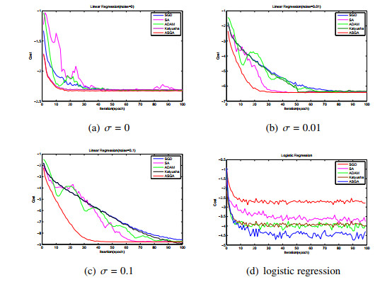
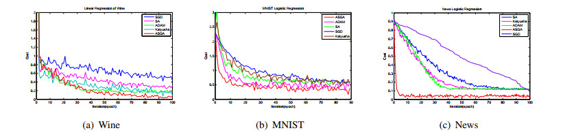
In this paper, we consider stochastic approximation algorithms for least-square and logistic regression with no strong-convexity assumption on the convex loss functions. We develop two algorithms with varied step-size motivated by the accelerated gradient algorithm which is initiated for convex stochastic programming. We analyse the developed algorithms that achieve a rate of $ O(1/n^{2}) $ where $ n $ is the number of samples, which is tighter than the best convergence rate $ O(1/n) $ achieved so far on non-strongly-convex stochastic approximation with constant-step-size, for classic supervised learning problems. Our analysis is based on a non-asymptotic analysis of the empirical risk (in expectation) with less assumptions that existing analysis results. It does not require the finite-dimensionality assumption and the Lipschitz condition. We carry out controlled experiments on synthetic and some standard machine learning data sets. Empirical results justify our theoretical analysis and show a faster convergence rate than existing other methods.
- least-square regression,
- logistic regression,
- accelerated stochastic approximation,
- convergence rate
Citation: Yiyuan Cheng, Yongquan Zhang, Xingxing Zha, Dongyin Wang. On stochastic accelerated gradient with non-strongly convexity[J]. AIMS Mathematics, 2022, 7(1): 1445-1459. doi: 10.3934/math.2022085

Related Papers:

Abstract

In this paper, we consider stochastic approximation algorithms for least-square and logistic regression with no strong-convexity assumption on the convex loss functions. We develop two algorithms with varied step-size motivated by the accelerated gradient algorithm which is initiated for convex stochastic programming. We analyse the developed algorithms that achieve a rate of $ O(1/n^{2}) $ where $ n $ is the number of samples, which is tighter than the best convergence rate $ O(1/n) $ achieved so far on non-strongly-convex stochastic approximation with constant-step-size, for classic supervised learning problems. Our analysis is based on a non-asymptotic analysis of the empirical risk (in expectation) with less assumptions that existing analysis results. It does not require the finite-dimensionality assumption and the Lipschitz condition. We carry out controlled experiments on synthetic and some standard machine learning data sets. Empirical results justify our theoretical analysis and show a faster convergence rate than existing other methods.

References

[1]	H. Robbins, S. Monro, A stochastic approximation method, In: The annals of mathematical statistics, Institute of Mathematical Statistics, 22 (1951), 400–407.
[2]	B. T. Polyak, New stochastic approximation type procedures, Automat. i Telemekh, 1990, 98–107.
[3]	B. T. Polyak, A. B. Juditsky, Acceleration of stochastic approximation by averaging, SIAM J. Control Optim., 30 (1992), 838–855. doi: 10.1137/0330046. doi: 10.1137/0330046
[4]	L. Bottou, O. Bousquet, The tradeoffs of large scale learning, In: Advances in neural information processing systems, 20 (2007), 1–8.
[5]	S. Shalev-Shwartz, Y. Singer, N. Srebro, A. Cotter, Pegasos: Primal estimated sub-gradient solver for SVM, Math. Program., 127 (2011), 3–30. doi: 10.1007/s10107-010-0420-4. doi: 10.1007/s10107-010-0420-4
[6]	A. Nemirovski, A. Juditsky, G. Lan, A. Shapiro, Robust stochastic approximation approach to stochastic programming, SIAM J. Optim., 19 (2009), 1574–1609. doi: 10.1137/070704277. doi: 10.1137/070704277
[7]	G. H. Lan, R. D. C. Monteiro, Iteration-complexity of first-order penalty methods for convex programming, Math. Program., 138 (2013), 115–139. doi: 10.1007/s10107-012-0588-x. doi: 10.1007/s10107-012-0588-x
[8]	S. Ghadimi, G. H. Lan, Accelerated gradient methods for nonconvex nonlinear and stochastic programming, Math. Program., 156 (2016), 59–99. doi: 10.1007/s10107-015-0871-8. doi: 10.1007/s10107-015-0871-8
[9]	F. Bach, E. Moulines, Non-asymptotic analysis of stochastic approximation algorithms for machine learning, 2011.
[10]	F. Bach, E. Moulines, Non-strongly-convex smooth stochastic approximation with convergence rate $O(1/n)$, 2013. Avaliable from: https://proceedings.neurips.cc/paper/2013/file/7fe1f8abaad094e0b5cb1b01d712f708-Paper.pdf.
[11]	J. C. Duchi, E. Hazan, Y. Singer, Adaptive subgradient methods for online learning and stochastic optimization, J. Mach. Learn. Res., 12 (2010), 2121–2159.
[12]	Y. E. Nesterov, A method of solving a convex programming problem with convergence rate $O(1/k^2)$, Dokl. Akad. Nauk SSSR, 269 (1983), 543–547.
[13]	A. Beck, M. Teboulle, A fast iterative shrinkage-thresholding algorithm for linear inverse problems, SIAM J. Imaging Sci., 2, (2009), 183–202. doi: 10.1137/080716542.
[14]	P. Tseng, On accelerated proximal gradient methods for convex-concave optimization, SIAM J. Optimiz., 2008.
[15]	Y. Nesterov, Smooth minimization of non-smooth functions, Math. Program., 103 (2005), 127–152. doi: 10.1007/s10107-004-0552-5. doi: 10.1007/s10107-004-0552-5
[16]	Y. Nesterov, Gradient methods for minimizing composite functions, Math. Program., 140 (2013), 125–161. doi: 10.1007/s10107-012-0629-5. doi: 10.1007/s10107-012-0629-5
[17]	G. H. Lan, An optimal method for stochastic composite optimization, Math. Program., 133 (2012), 365–397. doi: 10.1007/s10107-010-0434-y. doi: 10.1007/s10107-010-0434-y
[18]	S. Ghadimi, G. H. Lan, Optimal stochastic approximation algorithms for strongly convex stochastic composite optimization I: A generic algorithmic framework, SIAM J. Optim., 22 (2012), 1469–1492. doi: 10.1137/110848864. doi: 10.1137/110848864
[19]	S. Ghadimi, G. H. Lan, Stochastic first- and zeroth-order methods for nonconvex stochastic programming, SIAM J. Optim., 23 (2013), 2341–2368. doi: 10.1137/120880811. doi: 10.1137/120880811
[20]	S. Ghadimi, G. H. Lan, H. C. Zhang, Mini-batch stochastic approximation methods for nonconvex stochastic composite optimization, Math. Program., 155 (2016), 267–305. doi: 10.1007/s10107-014-0846-1. doi: 10.1007/s10107-014-0846-1
[21]	G. H. Lan, Bundle-level type methods uniformly optimal for smooth and nonsmooth convex optimization, Math. Program., 149 (2015), 1–45. doi: 10.1007/s10107-013-0737-x. doi: 10.1007/s10107-013-0737-x
[22]	S. Ghadimi, G. H. Lan, Accelerated gradient methods for nonconvex nonlinear and stochastic programming, Math. Program., 156 (2016), 59–99. doi: 10.1007/s10107-015-0871-8. doi: 10.1007/s10107-015-0871-8
[23]	L. Bottou, Large-scale machine learning with stochastic gradient descent. In: Proceedings of COMPSTAT'2010, Physica-Verlag HD, 2010,177–186. doi: 10.1007/978-3-7908-2604-3_16.
[24]	D. P. Kingma, J. Ba, Adam: A method for stochastic optimization, arXiv: 1412.6980v9, 2012.
[25]	Z. A. Zhu, Katyusha: The first direct acceleration of stochastic gradient methods, In: Proceedings of the 49th Annual ACM SIGACT Symposium on Theory of Computing (STOC 2017), New York, USA: Association for Computing Machinery. doi: 10.1145/3055399.3055448.

Reader Comments

Your name:*

Email:*
© 2022 the Author(s), licensee AIMS Press. This is an open access article distributed under the terms of the Creative Commons Attribution License (http://creativecommons.org/licenses/by/4.0)