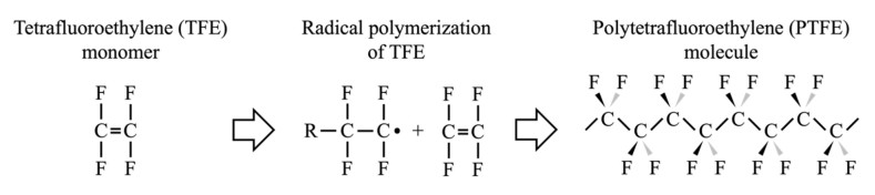
Polytetrafluoroethylene (PTFE) is a fully fluorinated linear polymer with a (CF2-CF2)n backbone. High molecular weight PTFEs are chemically inert while possessing excellent hydrophobic surface properties attributed to their low surface energy. These characteristics make PTFE an excellent candidate for membrane distillation application among all other hydrophobic polymers. In this review, the electrospinning processes of PTFE fibers are discussed in detail with a focus on various electrospinning effects on the resulting fiber morphologies and structures. Due to the high chemical resistance and low solvent solubility, PTFE is typically electrospin with a polymer carrier, such as polyvinyl alcohol (PVA) and/or polyethylene oxide (PEO), using emulsion electrospinning followed by a sintering process. The amount of PTFE in emulsion, types of polymer carriers, electrospinning parameters, and sintering conditions have interconnected effects on the resulting morphological structures of PFTE fibers (e.g., beading or continuous fibers). In addition, electrospun PTFE fibers are further functionalized using methods of co-electrospinning with other hydrophobic polymers as well as incorporations of metallic (ZnO) and inorganic particles (POSS) to improve their performance in membrane distillation. Water contact angles, permeation fluxes, salt rejection rates, and hours of operations are reported for various functionalized electrospun PTFE fibrous membranes to demonstrate their feasibility in membrane distillation applications. In general, this article provides a scientific understanding of electrospun PTFE fibers and their engineering application in membrane distillation.
Citation: Charles Defor, Shih-Feng Chou. Electrospun polytetrafluoroethylene (PTFE) fibers in membrane distillation applications[J]. AIMS Materials Science, 2024, 11(6): 1179-1198. doi: 10.3934/matersci.2024058
Polytetrafluoroethylene (PTFE) is a fully fluorinated linear polymer with a (CF2-CF2)n backbone. High molecular weight PTFEs are chemically inert while possessing excellent hydrophobic surface properties attributed to their low surface energy. These characteristics make PTFE an excellent candidate for membrane distillation application among all other hydrophobic polymers. In this review, the electrospinning processes of PTFE fibers are discussed in detail with a focus on various electrospinning effects on the resulting fiber morphologies and structures. Due to the high chemical resistance and low solvent solubility, PTFE is typically electrospin with a polymer carrier, such as polyvinyl alcohol (PVA) and/or polyethylene oxide (PEO), using emulsion electrospinning followed by a sintering process. The amount of PTFE in emulsion, types of polymer carriers, electrospinning parameters, and sintering conditions have interconnected effects on the resulting morphological structures of PFTE fibers (e.g., beading or continuous fibers). In addition, electrospun PTFE fibers are further functionalized using methods of co-electrospinning with other hydrophobic polymers as well as incorporations of metallic (ZnO) and inorganic particles (POSS) to improve their performance in membrane distillation. Water contact angles, permeation fluxes, salt rejection rates, and hours of operations are reported for various functionalized electrospun PTFE fibrous membranes to demonstrate their feasibility in membrane distillation applications. In general, this article provides a scientific understanding of electrospun PTFE fibers and their engineering application in membrane distillation.

| [1] |
Shyr TW, Chung WC, Lu WL, et al. (2015) Unusually high temperature transition and microporous structure of polytetrafluoroethylene fibre prepared through film fibrillation. Eur Polym J 72: 50–63. https://doi.org/10.1016/j.eurpolymj.2015.08.017 doi: 10.1016/j.eurpolymj.2015.08.017

|
| [2] |
Xu A, Li H, Yuan WZ, et al. (2012) Radical homopolymerization of tetrafluoroethylene initiated by perfluorodiacyl peroxide in supercritical carbon dioxide: Reaction mechanism and initiation kinetics. Eur Polym J 48: 1431–1438. https://doi.org/10.1016/j.eurpolymj.2012.05.012 doi: 10.1016/j.eurpolymj.2012.05.012
|
| [3] |
Clark ES (1999) The molecular conformations of polytetrafluoroethylene: Forms Ⅱ and Ⅳ. Polymer 40: 4659–4665. https://doi.org/10.1016/S0032-3861(99)00109-3 doi: 10.1016/S0032-3861(99)00109-3
|
| [4] |
Puts GJ, Crouse P, Ameduri BM (2019) Polytetrafluoroethylene: Synthesis and characterization of the original extreme polymer. Chem Rev 119: 1763–1805. https://doi.org/10.1021/acs.chemrev.8b00458 doi: 10.1021/acs.chemrev.8b00458
|
| [5] |
Biswas SK, Vijayan K (1992) Friction and wear of PTFE—A review. Wear 158: 193–211. https://doi.org/10.1016/0043-1648(92)90039-B doi: 10.1016/0043-1648(92)90039-B
|
| [6] |
Dhanumalayan E, Joshi GM (2018) Performance properties and applications of polytetrafluoroethylene (PTFE)—A review. Adv Compos Hybrid Mater 1: 247–268. https://doi.org/10.1007/s42114-018-0023-8 doi: 10.1007/s42114-018-0023-8
|
| [7] |
Lu X, Peng Y, Ge L, et al. (2016) Amphiphobic PVDF composite membranes for anti-fouling direct contact membrane distillation. J Membr Sci 505: 61–69. https://doi.org/10.1016/j.memsci.2015.12.042 doi: 10.1016/j.memsci.2015.12.042
|
| [8] |
Alessandro F, Macedonio F, Drioli E (2023) New materials and phenomena in membrane distillation. Chemistry 5: 65–84. https://doi.org/10.3390/chemistry5010006 doi: 10.3390/chemistry5010006
|
| [9] |
Li X, Yu X, Cheng C, et al. (2015) Electrospun superhydrophobic organic/inorganic composite nanofibrous membranes for membrane distillation. ACS Appl Mater Interfaces 7: 21919–21930. https://doi.org/10.1021/acsami.5b06509 doi: 10.1021/acsami.5b06509
|
| [10] |
Dong ZQ, Ma X, Xu ZL, et al. (2014) Superhydrophobic PVDF–PTFE electrospun nanofibrous membranes for desalination by vacuum membrane distillation. Desalination 347: 175–183. https://doi.org/10.1016/j.desal.2014.05.015 doi: 10.1016/j.desal.2014.05.015
|
| [11] |
Nthunya LN, Gutierrez L, Derese S, et al. (2019) A review of nanoparticle‐enhanced membrane distillation membranes: Membrane synthesis and applications in water treatment. J Chem Technol Biotechnol 94: 2757–2771. https://doi.org/10.1002/jctb.5977 doi: 10.1002/jctb.5977
|
| [12] |
Efome JE, Rana D, Matsuura T, et al. (2016) Enhanced performance of PVDF nanocomposite membrane by nanofiber coating: A membrane for sustainable desalination through MD. Water Res 89: 39–49. https://doi.org/10.1016/j.watres.2015.11.040 doi: 10.1016/j.watres.2015.11.040
|
| [13] |
Feng S, Zhong Z, Wang Y, et al. (2018) Progress and perspectives in PTFE membrane: Preparation, modification, and applications. J Membr Sci 549: 332–349. https://doi.org/10.1016/j.memsci.2017.12.032 doi: 10.1016/j.memsci.2017.12.032
|
| [14] |
Huang QL, Xiao C, Feng X, et al. (2013) Design of super-hydrophobic microporous polytetrafluoroethylene membranes. New J Chem 37: 373–379. https://doi.org/10.1039/C2NJ40355B doi: 10.1039/C2NJ40355B
|
| [15] |
Li L, Sirkar KK (2016) Influence of microporous membrane properties on the desalination performance in direct contact membrane distillation. J Membr Sci 513: 280–293. https://doi.org/10.1021/acsami.5b06509 doi: 10.1021/acsami.5b06509
|
| [16] |
Yang Y, Strobel M, Kirk S, et al. (2010) Fluorine plasma treatments of poly(propylene) films, 2—Modeling reaction mechanisms and scaling. Plasma Process Polym 7: 123–150. https://doi.org/10.1002/ppap.200900114 doi: 10.1002/ppap.200900114
|
| [17] |
Bottino A, Capannelli G, Comite A, et al. (2015) Novel polytetrafluoroethylene tubular membranes for membrane distillation. Desalination Water Treat 53: 1559–1564. https://doi.org/10.1080/19443994.2014.982955 doi: 10.1080/19443994.2014.982955
|
| [18] | Reza Shirzad Kebria M, Rahimpour A (2020) Membrane distillation: Basics, advances, and applications, In: Abdelrasoul A, Advances in Membrane Technologies, Rijeka: IntechOpen, 67–87. https://doi.org/10.5772/intechopen.86952 |
| [19] |
Xu H, Jin W, Wang F, et al. (2018) Preparation and properties of PTFE hollow fiber membranes for the removal of ultrafine particles in PM2.5 with repetitive usage capability. RSC Adv 8: 38245–38258. https://doi.org/10.1039/C8RA07789D doi: 10.1039/C8RA07789D
|
| [20] |
Lu W, Yuan Z, Zhao Y, et al. (2017) Porous membranes in secondary battery technologies. Chem Soc Rev 46: 2199–2236. https://doi.org/10.1039/C6CS00823B doi: 10.1039/C6CS00823B
|
| [21] |
Gu M, Zhang J, Wang X, et al. (2006) Formation of poly(vinylidene fluoride) (PVDF) membranes via thermally induced phase separation. Desalination 192: 160–167. https://doi.org/10.1016/j.desal.2005.10.015 doi: 10.1016/j.desal.2005.10.015
|
| [22] |
Karimi H, Rahimpour A, Shirzad Kebria MR (2016) Pesticides removal from water using modified piperazine-based nanofiltration (NF) membranes. Desalination Water Treat 57: 24844–24854. https://doi.org/10.1080/19443994.2016.1156580 doi: 10.1080/19443994.2016.1156580
|
| [23] | Mahdi A Shirazi M, Bazgir S, Meshkani F (2020) Electrospun nanofibrous membranes for water treatment, In: Abdelrasoul A, Advances in Membrane Technologies, Rijeka: IntechOpen. https://doi.org/10.5772/intechopen.87948 |
| [24] | Shirazi MMA, Asghari M (2018) Electrospun filters for oil–water separation, In: Focarete ML, Gualandi C, Ramakrishna S, Filtering Media by Electrospinning, Cham: Springer International Publishing, 151–173. https://doi.org/10.1007/978-3-319-78163-1_7 |
| [25] |
Emerine R, Chou SF (2022) Fast delivery of melatonin from electrospun blend polyvinyl alcohol and polyethylene oxide (PVA/PEO) fibers. AIMS Bioeng 9: 178–196. https://doi.org/10.3934/bioeng.2022013 doi: 10.3934/bioeng.2022013
|
| [26] |
Hawkins BC, Burnett E, Chou SF (2022) Physicomechanical properties and in vitro release behaviors of electrospun ibuprofen-loaded blend PEO/EC fibers. Mater Today Commun 30: 103205. https://doi.org/10.1016/j.mtcomm.2022.103205 doi: 10.1016/j.mtcomm.2022.103205
|
| [27] |
Faglie A, Emerine R, Chou SF (2023) Effects of poloxamers as excipients on the physicomechanical properties, cellular biocompatibility, and in vitro drug release of electrospun polycaprolactone (PCL) fibers. Polymers 15: 2997. https://doi.org/10.3390/polym15142997 doi: 10.3390/polym15142997
|
| [28] |
Gizaw M, Bani Mustafa D, Chou SF (2023) Fabrication of drug-eluting polycaprolactone and chitosan blend microfibers for topical drug delivery applications. Front Mater 10: 1144752. https://doi.org/10.3389/fmats.2023.1144752 doi: 10.3389/fmats.2023.1144752
|
| [29] |
Bani Mustafa D, Sakai T, Sato O, et al. (2024) Electrospun ibuprofen-loaded blend PCL/PEO fibers for topical drug delivery applications. Polymers 16: 1934. https://doi.org/10.3390/polym16131934 doi: 10.3390/polym16131934
|
| [30] |
Mohamed R, Chou SF (2024) Physicomechanical characterizations and in vitro release studies of electrospun ethyl cellulose fibers, solvent cast carboxymethyl cellulose films, and their composites. Int J Biol Macromol 267: 131374. https://doi.org/10.1016/j.ijbiomac.2024.131374 doi: 10.1016/j.ijbiomac.2024.131374
|
| [31] |
Subbiah T, Bhat GS, Tock RW, et al. (2005) Electrospinning of nanofibers. J Appl Polym Sci 96: 557–569. https://doi.org/10.1002/app.21481 doi: 10.1002/app.21481
|
| [32] | Formhals A (1934) Process and apparatus for preparing artificial threads. |
| [33] |
Taylor GI (1969) Electrically driven jets. Proc R Soc Lond Math Phys Sci 313: 453–475. https://doi.org/10.1098/rspa.1969.0205 doi: 10.1098/rspa.1969.0205
|
| [34] |
Huang ZM, Zhang YZ, Kotaki M, et al. (2003) A review on polymer nanofibers by electrospinning and their applications in nanocomposites. Compos Sci Technol 63: 2223–2253. https://doi.org/10.1016/S0266-3538(03)00178-7 doi: 10.1016/S0266-3538(03)00178-7
|
| [35] |
Wang X, Hsiao BS (2016) Electrospun nanofiber membranes. Curr Opin Chem Eng 12: 62–81. https://doi.org/10.1016/j.coche.2016.03.001 doi: 10.1016/j.coche.2016.03.001
|
| [36] |
Beachley V, Wen X (2009) Effect of electrospinning parameters on the nanofiber diameter and length. Mater Sci Eng C 29: 663–668. https://doi.org/10.1016/j.msec.2008.10.037 doi: 10.1016/j.msec.2008.10.037
|
| [37] |
Yördem OS, Papila M, Menceloğlu YZ (2008) Effects of electrospinning parameters on polyacrylonitrile nanofiber diameter: An investigation by response surface methodology. Mater Des 29: 34–44. https://doi.org/10.1016/j.matdes.2006.12.013 doi: 10.1016/j.matdes.2006.12.013
|
| [38] |
Zhang C, Yuan X, Wu L, et al. (2005) Study on morphology of electrospun poly(vinyl alcohol) mats. Eur Polym J 41: 423–432. https://doi.org/10.1016/j.eurpolymj.2004.10.027 doi: 10.1016/j.eurpolymj.2004.10.027
|
| [39] |
Zargham S, Bazgir S, Tavakoli A, et al. (2012) The effect of flow rate on morphology and deposition area of electrospun nylon 6 nanofiber. J Eng Fibers Fabr 7: 42–49. https://doi.org/10.1177/155892501200700414 doi: 10.1177/155892501200700414
|
| [40] |
Homayoni H, Ravandi SAH, Valizadeh M (2009) Electrospinning of chitosan nanofibers: Processing optimization. Carbohydr Polym 77: 656–661. https://doi.org/10.1016/j.carbpol.2009.02.008 doi: 10.1016/j.carbpol.2009.02.008
|
| [41] |
Tan SH, Inai R, Kotaki M, et al. (2005) Systematic parameter study for ultra-fine fiber fabrication via electrospinning process. Polymer 46: 6128–6134. https://doi.org/10.1016/j.polymer.2005.05.068 doi: 10.1016/j.polymer.2005.05.068
|
| [42] |
Liu Y, He J, Yu J, et al. (2008) Controlling numbers and sizes of beads in electrospun nanofibers. Polym Int 57: 632–636. https://doi.org/10.1002/pi.2387 doi: 10.1002/pi.2387
|
| [43] |
He JH, Wan YQ, Yu JY (2008) Effect of concentration on electrospun polyacrylonitrile (PAN) nanofibers. Fibers Polym 9: 140–142. https://doi.org/10.1007/s12221-008-0023-3 doi: 10.1007/s12221-008-0023-3
|
| [44] |
Koski A, Yim K, Shivkumar S (2004) Effect of molecular weight on fibrous PVA produced by electrospinning. Mater Lett 58: 493–497. https://doi.org/10.1016/S0167-577X(03)00532-9 doi: 10.1016/S0167-577X(03)00532-9
|
| [45] |
Mit‐uppatham C, Nithitanakul M, Supaphol P (2004) Ultrafine electrospun polyamide‐6 fibers: Effect of solution conditions on morphology and average fiber diameter. Macromol Chem Phys 205: 2327–2338. https://doi.org/10.1002/macp.200400225 doi: 10.1002/macp.200400225
|
| [46] |
Jarusuwannapoom T, Hongrojjanawiwat W, Jitjaicham S, et al. (2005) Effect of solvents on electro-spinnability of polystyrene solutions and morphological appearance of resulting electrospun polystyrene fibers. Eur Polym J 41: 409–421. https://doi.org/10.1016/j.eurpolymj.2004.10.010 doi: 10.1016/j.eurpolymj.2004.10.010
|
| [47] |
Jia L, Qin X (2013) The effect of different surfactants on the electrospinning poly(vinyl alcohol) (PVA) nanofibers. J Therm Anal Calorim 112: 595–605. https://doi.org/10.1007/s10973-012-2607-9 doi: 10.1007/s10973-012-2607-9
|
| [48] |
Fan L, Xu Y, Zhou X, et al. (2018) Effect of salt concentration in spinning solution on fiber diameter and mechanical property of electrospun styrene-butadiene-styrene tri-block copolymer membrane. Polymer 153: 61–69. https://doi.org/10.1016/j.polymer.2018.08.008 doi: 10.1016/j.polymer.2018.08.008
|
| [49] |
Qin X, Yang E, Li N, et al. (2007) Effect of different salts on electrospinning of polyacrylonitrile (PAN) polymer solution. J Appl Polym Sci 103: 3865–3870. https://doi.org/10.1002/app.25498 doi: 10.1002/app.25498
|
| [50] |
Uyar T, Besenbacher F (2008) Electrospinning of uniform polystyrene fibers: The effect of solvent conductivity. Polymer 49: 5336–5343. https://doi.org/10.1016/j.polymer.2008.09.025 doi: 10.1016/j.polymer.2008.09.025
|
| [51] |
Tungprapa S, Puangparn T, Weerasombut M, et al. (2007) Electrospun cellulose acetate fibers: Effect of solvent system on morphology and fiber diameter. Cellulose 14: 563–575. https://doi.org/10.1007/s10570-007-9113-4 doi: 10.1007/s10570-007-9113-4
|
| [52] |
Huan S, Liu G, Han G, et al. (2015) Effect of experimental parameters on morphological, mechanical and hydrophobic properties of electrospun polystyrene fibers. Materials 8: 2718–2734. https://doi.org/10.3390/ma8052718 doi: 10.3390/ma8052718
|
| [53] |
Moomand K, Lim LT (2015) Effects of solvent and n-3 rich fish oil on physicochemical properties of electrospun zein fibres. Food Hydrocoll 46: 191–200. https://doi.org/10.1016/j.foodhyd.2014.12.014 doi: 10.1016/j.foodhyd.2014.12.014
|
| [54] |
Song Z, Chiang SW, Chu X, et al. (2018) Effects of solvent on structures and properties of electrospun poly(ethylene oxide) nanofibers. J Appl Polym Sci 135: 45787. https://doi.org/10.1002/app.45787 doi: 10.1002/app.45787
|
| [55] |
De Vrieze S, Van Camp T, Nelvig A, et al. (2009) The effect of temperature and humidity on electrospinning. J Mater Sci 44: 1357–1362. https://doi.org/10.1007/s10853-008-3010-6 doi: 10.1007/s10853-008-3010-6
|
| [56] |
Hardick O, Stevens B, Bracewell DG (2011) Nanofibre fabrication in a temperature and humidity controlled environment for improved fibre consistency. J Mater Sci 46: 3890–3898. https://doi.org/10.1007/s10853-011-5310-5 doi: 10.1007/s10853-011-5310-5
|
| [57] |
Hunke H, Soin N, Shah T, et al. (2015) Influence of plasma pre-treatment of polytetrafluoroethylene (PTFE) micropowders on the mechanical and tribological performance of polyethersulfone (PESU)–PTFE composites. Wear 328–329: 480–487. https://doi.org/10.1016/j.wear.2015.03.004 doi: 10.1016/j.wear.2015.03.004
|
| [58] |
Hunke H, Soin N, Shah T, et al. (2015) Low-pressure H2, NH3 microwave plasma treatment of polytetrafluoroethylene (PTFE) powders: Chemical, thermal and wettability analysis. Materials 8: 2258–2275. https://doi.org/10.3390/ma8052258 doi: 10.3390/ma8052258
|
| [59] |
Zhao P, Soin N, Prashanthi K, et al. (2018) Emulsion electrospinning of polytetrafluoroethylene (PTFE) nanofibrous membranes for high-performance triboelectric nanogenerators. ACS Appl Mater Interfaces 10: 5880–5891. https://doi.org/10.1021/acsami.7b18442 doi: 10.1021/acsami.7b18442
|
| [60] |
Yazgan G, Popa AM, Rossi RM, et al. (2015) Tunable release of hydrophilic compounds from hydrophobic nanostructured fibers prepared by emulsion electrospinning. Polymer 66: 268–276. https://doi.org/10.1016/j.polymer.2015.04.045 doi: 10.1016/j.polymer.2015.04.045
|
| [61] |
Akduman C (2023) Preparation and comparison of electrospun PEO/PTFE and PVA/PTFE nanofiber membranes for syringe filters. J Appl Polym Sci 140: e54344. https://doi.org/10.1002/app.54344 doi: 10.1002/app.54344
|
| [62] |
Qing W, Shi X, Deng Y, et al. (2017) Robust superhydrophobic-superoleophilic polytetrafluoroethylene nanofibrous membrane for oil/water separation. J Membr Sci 540: 354–361. https://doi.org/10.1016/j.memsci.2017.06.060 doi: 10.1016/j.memsci.2017.06.060
|
| [63] |
Xiong J, Huo P, Ko FK (2009) Fabrication of ultrafine fibrous polytetrafluoroethylene porous membranes by electrospinning. J Mater Res 24: 2755–2761. https://doi.org/10.1557/jmr.2009.0347 doi: 10.1557/jmr.2009.0347
|
| [64] |
Su C, Li Y, Cao H, et al. (2019) Novel PTFE hollow fiber membrane fabricated by emulsion electrospinning and sintering for membrane distillation. J Membr Sci 583: 200–208. https://doi.org/10.1016/j.memsci.2019.04.037 doi: 10.1016/j.memsci.2019.04.037
|
| [65] |
Son SJ, Hong SK, Lim G (2020) Emulsion electrospinning of hydrophobic PTFE-PEO composite nanofibrous membranes for simple oil/water separation. J Sens Sci Technol 29: 89–92. https://doi.org/10.5369/JSST.2020.29.2.89 doi: 10.5369/JSST.2020.29.2.89
|
| [66] |
Cheng J, Huang Q, Huang Y, et al. (2020) Study on a novel PTFE membrane with regular geometric pore structures fabricated by near-field electrospinning, and its applications. J Membr Sci 603: 118014. https://doi.org/10.1016/j.memsci.2020.118014 doi: 10.1016/j.memsci.2020.118014
|
| [67] |
Kianfar P, Bongiovanni R, Ameduri B, et al. (2023) Electrospinning of fluorinated polymers: Current state of the art on processes and applications. Polym Rev 63: 127–199. https://doi.org/10.1080/15583724.2022.2067868 doi: 10.1080/15583724.2022.2067868
|
| [68] |
Han D, Steckl AJ (2009) Superhydrophobic and oleophobic fibers by coaxial electrospinning. Langmuir 25: 9454–9462. https://doi.org/10.1021/la900660v doi: 10.1021/la900660v
|
| [69] |
Feng C, Khulbe KC, Matsuura T, et al. (2008) Production of drinking water from saline water by air-gap membrane distillation using polyvinylidene fluoride nanofiber membrane. J Membr Sci 311: 1–6. https://doi.org/10.1016/j.memsci.2007.12.026 doi: 10.1016/j.memsci.2007.12.026
|
| [70] |
Prince JA, Singh G, Rana D, et al. (2012) Preparation and characterization of highly hydrophobic poly(vinylidene fluoride)—Clay nanocomposite nanofiber membranes (PVDF–clay NNMs) for desalination using direct contact membrane distillation. J Membr Sci 397–398: 80–86. https://doi.org/10.1016/j.memsci.2012.01.012 doi: 10.1016/j.memsci.2012.01.012
|
| [71] |
Wang P, Chung TS (2015) Recent advances in membrane distillation processes: Membrane development, configuration design and application exploring. J Membr Sci 474: 39–56. https://doi.org/10.1016/j.memsci.2014.09.016 doi: 10.1016/j.memsci.2014.09.016
|
| [72] |
Singh S, Mahalingam H, Singh PK (2013) Polymer-supported titanium dioxide photocatalysts for environmental remediation: A review. Appl Catal Gen 462–463: 178–195. https://doi.org/10.1016/j.apcata.2013.04.039 doi: 10.1016/j.apcata.2013.04.039
|
| [73] |
Pei CC, Leung WWF (2013) Enhanced photocatalytic activity of electrospun TiO2/ZnO nanofibers with optimal anatase/rutile ratio. Catal Commun 37: 100–104. https://doi.org/10.1016/j.catcom.2013.03.029 doi: 10.1016/j.catcom.2013.03.029
|
| [74] |
Sankapal BR, Lux-Steiner MCh, Ennaoui A (2005) Synthesis and characterization of anatase-TiO2 thin films. Appl Surf Sci 239: 165–170. https://doi.org/10.1016/j.apsusc.2004.05.142 doi: 10.1016/j.apsusc.2004.05.142
|
| [75] |
Bozzi A, Yuranova T, Kiwi J (2005) Self-cleaning of wool-polyamide and polyester textiles by TiO2-rutile modification under daylight irradiation at ambient temperature. J Photochem Photobiol Chem 172: 27–34. https://doi.org/10.1016/j.jphotochem.2004.11.010 doi: 10.1016/j.jphotochem.2004.11.010
|
| [76] |
Huang QL, Huang Y, Xiao CF, et al. (2017) Electrospun ultrafine fibrous PTFE-supported ZnO porous membrane with self-cleaning function for vacuum membrane distillation. J Membr Sci 534: 73–82. https://doi.org/10.1016/j.memsci.2017.04.015 doi: 10.1016/j.memsci.2017.04.015
|
| [77] |
Saffarini RB, Mansoor B, Thomas R, et al. (2013) Effect of temperature-dependent microstructure evolution on pore wetting in PTFE membranes under membrane distillation conditions. J Membr Sci 429: 282–294. https://doi.org/10.1016/j.memsci.2012.11.049 doi: 10.1016/j.memsci.2012.11.049
|
| [78] |
Xu M, Cheng J, Du X, et al. (2022) Amphiphobic electrospun PTFE nanofibrous membranes for robust membrane distillation process. J Membr Sci 641: 119876. https://doi.org/10.1016/j.memsci.2021.119876 doi: 10.1016/j.memsci.2021.119876
|
| [79] |
Ju J, Fejjari K, Cheng Y, et al. (2020) Engineering hierarchically structured superhydrophobic PTFE/POSS nanofibrous membranes for membrane distillation. Desalination 486: 114481. https://doi.org/10.1016/j.desal.2020.114481 doi: 10.1016/j.desal.2020.114481
|
| [80] |
Lu C, Su C, Cao H, et al. (2018) F-POSS based omniphobic membrane for robust membrane distillation. Mater Lett 228: 85–88. https://doi.org/10.1016/j.matlet.2018.05.126 doi: 10.1016/j.matlet.2018.05.126
|
| [81] |
Bharadwaj RK, Berry RJ, Farmer BL (2000) Molecular dynamics simulation study of norbornene–POSS polymers. Polymer 41: 7209–7221. https://doi.org/10.1016/S0032-3861(00)00072-0 doi: 10.1016/S0032-3861(00)00072-0
|
| [82] |
Liu Y, Meng Z, Zou R, et al. (2024) Crosslinking and fluorination reinforced PTFE nanofibrous membrane with excellent amphiphobic performance for low-scaling membrane distillations. Water Res 256: 121594. https://doi.org/10.1016/j.watres.2024.121594 doi: 10.1016/j.watres.2024.121594
|


Figures(4) / Tables(2)

Charles Defor, Shih-Feng Chou. Electrospun polytetrafluoroethylene (PTFE) fibers in membrane distillation applications[J]. AIMS Materials Science, 2024, 11(6): 1179-1198. doi: 10.3934/matersci.2024058


 DownLoad: