Heat input effects on mechanical constraints and microstructural constituents of MAG and laser 316L austenitic stainless-steel welded joints

Francois Njock Bayock; Paul Kah; Kibong Marius Tony; Francois Njock Bayock; Paul Kah; Kibong Marius Tony

doi:10.3934/matersci.2022014

AIMS Materials Science

2022, Volume 9, Issue 2: 236-254. doi: 10.3934/matersci.2022014

Previous Article Next Article

Research article Special Issues

Heat input effects on mechanical constraints and microstructural constituents of MAG and laser 316L austenitic stainless-steel welded joints

1.
Department of Mechanical Engineering, ENSET Douala, University of Douala, P.O. Box: 1872, Douala, Cameroon
2.
Department of Engineering Science, University West, Gustava Melius gata 2 S-461 32 Trollhättan, Sweden
3.
Laboratory of Technologies and Applied Sciences, University Institute of Technology, University of Douala, PO Box 8698 Douala, Cameroon

Received: 15 November 2021 Revised: 30 January 2022 Accepted: 17 February 2022 Published: 22 February 2022

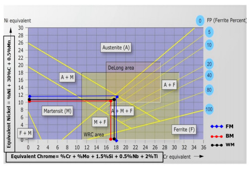
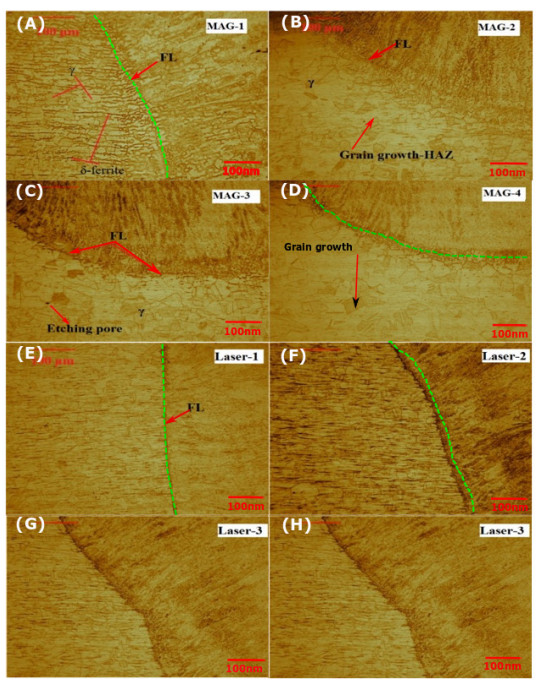
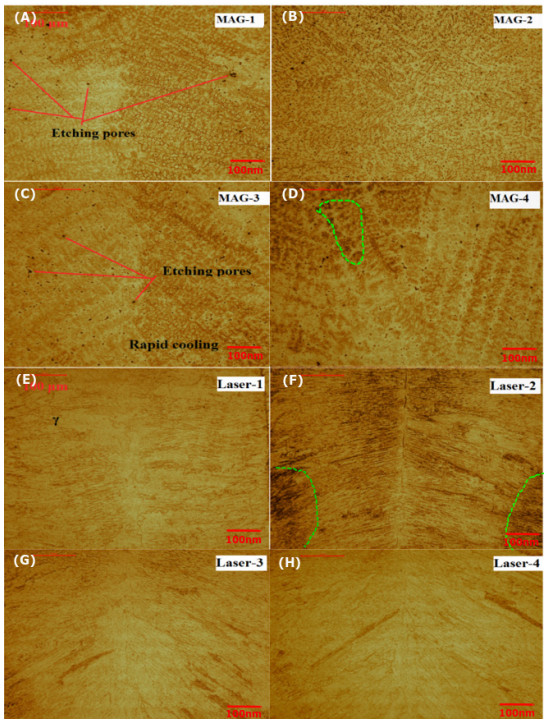
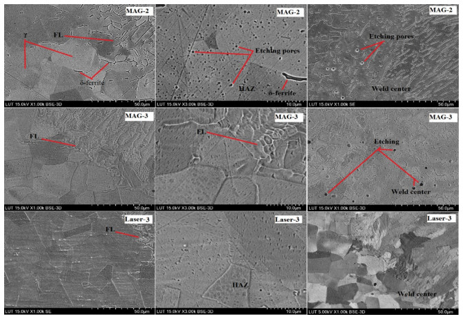
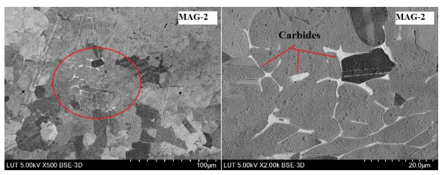
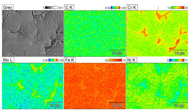
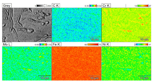
This study aims to investigate the optimum heat input required to overcome the negative consequence of the thermal properties of austenitic stainless steel to produce welded joints free of distortion. An experimental investigation using robotic-MAG and fiber-laser welding processes has been used in other to investigate angular, longitudinal distortion (bending), and microstructural constituents in the heat-affected zone (HAZ) of different welded joints. Ten 316L steel, butt-joints were made by different travel 25 speeds at the range of (7–11 mm/s). A highly sensitive 2D-laser device has been used to measure the distortion then, a microstructural investigation was done using an optical micrograph, Scanning Electron Microscopy (SEM) coupled with the Electron Dispersive Spectrometer (EDS). The laser-fiber welding process results indicated optimum parameters to prevent distortion when applying welding speed of 2.2 m/min, the power source of 2.5 kW, and the focal position of 3 mm. In MAG welding, test results revealed an increase of longitudinal distortion (bending) from 1.2 mm to 3.6 mm when raising the heat input from 0.3 to 0.472 kJ/mm. When increases welding speed (11 mm/s), angular distortion was approximately 2.1° on the left side and 1.7° on the right side. Microstructural investigations revealed the proportionality between heat input and carbides formations on the grain boundaries of HAZ. They were also the formation of etching pores and some ferrite content (10%) on the weld center.
- heat input,
- angular distortion,
- hot cracking,
- microstructural constituent longitudinal distortion,
- 316L stainless steel,
- SEM,
- EDS microscopy
Citation: Francois Njock Bayock, Paul Kah, Kibong Marius Tony. Heat input effects on mechanical constraints and microstructural constituents of MAG and laser 316L austenitic stainless-steel welded joints[J]. AIMS Materials Science, 2022, 9(2): 236-254. doi: 10.3934/matersci.2022014

Related Papers:

Abstract

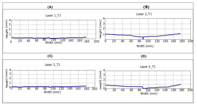
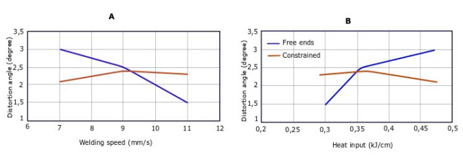
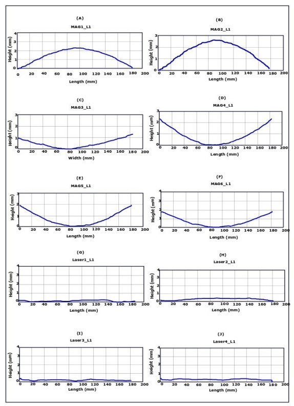
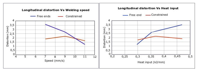
This study aims to investigate the optimum heat input required to overcome the negative consequence of the thermal properties of austenitic stainless steel to produce welded joints free of distortion. An experimental investigation using robotic-MAG and fiber-laser welding processes has been used in other to investigate angular, longitudinal distortion (bending), and microstructural constituents in the heat-affected zone (HAZ) of different welded joints. Ten 316L steel, butt-joints were made by different travel 25 speeds at the range of (7–11 mm/s). A highly sensitive 2D-laser device has been used to measure the distortion then, a microstructural investigation was done using an optical micrograph, Scanning Electron Microscopy (SEM) coupled with the Electron Dispersive Spectrometer (EDS). The laser-fiber welding process results indicated optimum parameters to prevent distortion when applying welding speed of 2.2 m/min, the power source of 2.5 kW, and the focal position of 3 mm. In MAG welding, test results revealed an increase of longitudinal distortion (bending) from 1.2 mm to 3.6 mm when raising the heat input from 0.3 to 0.472 kJ/mm. When increases welding speed (11 mm/s), angular distortion was approximately 2.1° on the left side and 1.7° on the right side. Microstructural investigations revealed the proportionality between heat input and carbides formations on the grain boundaries of HAZ. They were also the formation of etching pores and some ferrite content (10%) on the weld center.

References

[1]	International Stainless Steel Forum (ISSF), Stainless steel in figures, 2020. Available from: https://www.worldstainless.org.
[2]	Outokumpu Oyi (2013) Hanbook of Stainless Steel, Finland: Outokumpu Oyi.
[3]	Ezer M, Cam G (2020) Investigation of the microstructure and mechanical properties of gas metal arc welded AISI 304 austenitic stainless steel butt joints, In: Çınar Ö, 2020 Proceedings of International Conference on Engineering Technology and Innovation (ICETI), 1–10.
[4]	Şenol M, Cam G (2020) Microstructural and mechanical characterization of gas metal arc welded AISI 430 ferritic stainless steel joints, In: Çınar Ö, 2020 Proceedings of International Conference on Engineering Technology and Innovation (ICETI), 11–19.
[5]	Serindağ H, Çam G (2021) Microstructure and mechanical properties of gas metal arc welded AISI 430/AISI 304 dissimilar stainless steels butt joints. JPCS 1777: 012047. https://doi.org/10.1088/1742-6596/1777/1/012047 doi: 10.1088/1742-6596/1777/1/012047
[6]	Çam G, Yeni Ç, Erim S, et al. (1998) Investigation into properties of laser-welded similar and dissimilar steel joints. Sci Technol Weld Joi 3: 177-189. https://doi.org/10.1179/stw.1998.3.4.177 doi: 10.1179/stw.1998.3.4.177
[7]	Çam G, Erim S, Yeni Ç, et al. (1999) Determination of mechanical and fracture properties of laser beam welded steel joints. Weld J 78: 193s-201s.
[8]	Çam G (2011) Friction stir welded structural materials: Beyond Al-alloys. Int Mater Rev 56: 1–8. https://doi.org/10.1179/095066010X12777205875750 doi: 10.1179/095066010X12777205875750
[9]	Çam G, İpekoğlu G, Küçükömeroğlu T, et al. (2017) Applicability of friction stir welding to steels. JAMME 80: 65–85. https://doi.org/10.5604/01.3001.0010.2027 doi: 10.5604/01.3001.0010.2027
[10]	Yavuz H, Çam G (2005) Laser-arc hybrid welding method. Eng and Mach 46: 14–19.
[11]	Raden D, Kariem A, Neswan O, et al. (2019) Mechanical properties and microstructure at stainless steel HAZ from dissimilar metal welding after heat treatment processes. IOP Conf Series Mater Sci Eng 553: 012034. https://doi.org/10.1088/1757-899X/553/1/012034 doi: 10.1088/1757-899X/553/1/012034
[12]	Cao L, Shao X, Jiang P, et al. (2017) Effects of welding speed on microstructure and mechanical property of fiber laser welded dissimilar butt joints between AISI316L and EH36. Metals 7: 1–13. https://doi.org/10.3390/met7070270 doi: 10.3390/met7070270
[13]	Grigorenko G, Kostin A (2013) Criteria for evaluating the weldability of steels. Weld Int 27: 815–820. https://doi.org/10.1080/09507116.2013.796633 doi: 10.1080/09507116.2013.796633
[14]	Demarque R, Dos Santos E, Silva R, et al. (2018) Evaluation of the effect of the thermal cycle on the characteristics of welded joints through the variation of the heat input of the austenitic AISI 316L steels by the GMAW process. Sci Technology Mater 30: 51–59. https://doi.org/10.1016/j.stmat.2018.09.001 doi: 10.1016/j.stmat.2018.09.001
[15]	Jafarzadegan M, Feng H, Abdollah-zadeh A, et al. (2012) Microstructural characterization in dissimilar friction stir welding between 304 stainless steel and st37 steel. Mater Charact 74: 28–41. https://doi.org/10.1016/j.matchar.2012.09.004 doi: 10.1016/j.matchar.2012.09.004
[16]	Lippold J (2014) Welding Metallurgy and Weldability, 1 Ed., John Wiley & Sons. https://doi.org/10.1002/9781118960332
[17]	Landowski M, Swierczynska A, Rogalski G, et al. (2020) Autogenous fiber laser welding of 316L austenitic and 2304 lean duplex stainless steels. Materials 13: 2930. https://doi.org/10.3390/ma13132930 doi: 10.3390/ma13132930
[18]	Rogalski G, Swierczynska A, Landowski M, et al. (2020) Mechanical and microstructural characterization of TIG welded dissimilar joint between 304L austenitic stainless steel and Incoloy 800HT nickel alloy. Metals 10: 559. https://doi.org/10.3390/met10050559 doi: 10.3390/met10050559
[19]	Dong L, Zhang X, Han Y, Peng Q, et al. (2020) Effect of surface treatments on microstructure and stress corrosion cracking behaviour of 308L weld metal in a primary pressurized water reactor environment. Corros Sci 166: 108465. https://doi.org/10.1016/j.corsci.2020.108465 doi: 10.1016/j.corsci.2020.108465
[20]	Kumar K, Ramkumar D, Arivazhagan N (2015) Characterization of metallurgical and mechanical properties on the multi-pass welding of Inconel 625 and AISI 316L. J Mech Sci Technol 29: 1039–1047. https://doi.org/10.1007/s12206-014-1112-4 doi: 10.1007/s12206-014-1112-4
[21]	Ramkumar D, Reddy M, Arjun R, et al. (2015) Effect of filler metals on the weldability and mechanical properties of multi-pass PCGTA weldments of AISI 316L. J Mater Eng Perform 24: 1602–1613. https://doi.org/10.1007/s11665-015-1418-0 doi: 10.1007/s11665-015-1418-0
[22]	Shankar V, Gill T, Mannan L, et al. (2003) Effect of nitrogen addition on microstructure and fusion zone cracking in type 316L stainless steel weld metals. Mat Sci Eng A-Struct A343: 170–181. https://doi.org/10.1016/S0921-5093(02)00377-5 doi: 10.1016/S0921-5093(02)00377-5
[23]	Younes C, Steele A, Nicholson J, et al. (2013) Influence of hydrogen content on the tensile properties and fracture of austenitic stainless steel welds. Int Hydrogen Energ 38: 4864–4876. https://doi.org/10.1016/j.ijhydene.2012.11.016 doi: 10.1016/j.ijhydene.2012.11.016
[24]	Sadeghan M, Shamanian M, Shafyei A, et al. (2014) Effect of heat on microstructure and mechanical properties of dissimilar joints between super duplex stainless steel and high strength low alloy steel. Mater Design 60: 678–684. https://doi.org/10.1016/j.matdes.2014.03.057 doi: 10.1016/j.matdes.2014.03.057
[25]	Ramdan R, Koswara A, Wirawan R, et al. (2018) Metallurgy and mechanical properties variation with heat input, during dissimilar metal welding between stainless and carbon steel. IOP Conf Ser Mater Sci Eng 307: 012056. https://doi.org/10.1088/1757-899X/307/1/012056 doi: 10.1088/1757-899X/307/1/012056
[26]	Pazooki A, Hermans M, Richardson I (2017) Control of welding distortion during gas metal arc welding of AH36 plates by stress engineering. Int Adv Manuf Tech 88: 1439–1457. https://doi.org/10.1007/s00170-016-8869-9 doi: 10.1007/s00170-016-8869-9
[27]	Adamczuk P, Machado I, Mazzaferro J (2017) Methodology for predicting the angular distortion in multi-pass butt-joint welding. J Mater Process Tech 240: 305-313. https://doi.org/10.1016/j.jmatprotec.2016.10.006 doi: 10.1016/j.jmatprotec.2016.10.006
[28]	Mvola B, Kah P (2017) Effects of shielding gas control: welded joint properties in GMAW process optimization. Int Adv Manuf Tech 88: 2369–2387. https://doi.org/10.1007/s00170-016-8936-2 doi: 10.1007/s00170-016-8936-2
[29]	Kaneko K, Fukunaga T, Yamada K, et al. (2011) Formation of M23C6-type precipitates and chromium-depleted zones in austenite stainless steel. Scripta Mater 65: 509–512. https://doi.org/10.1016/j.scriptamat.2011.06.010 doi: 10.1016/j.scriptamat.2011.06.010
[30]	Kozuh S, Gojic M, Kosec L (2009) Mechanical properties and microstructure of austenitic stainless after welding and post-weld heat treatment. Kovove Mater 47: 253–262.
[31]	Parvathavarthini N, Dayal R, Hhatak H, et al. (2006) Sensitization behavior of modified 316N and 316L stainless steel weld metals after complexannealing and stress relieving cycles. J Nucl Mater 355: 68–82. https://doi.org/10.1016/j.jnucmat.2006.04.006 doi: 10.1016/j.jnucmat.2006.04.006
[32]	Ghusoon R, Ishak M, Aqida S, et al. (2017) Weld bead profile of laser welding dissimilar joints stainless steel. IOP Conf Ser Mater Sci Eng 257: 012072 https://doi.org/10.1088/1757-899X/257/1/012072 doi: 10.1088/1757-899X/257/1/012072
[33]	Mani C, Karthikeyan R, Vincent S (2018) A study on corrosion resistance of dissimilar welds between Monel 400 and 316L austenitic steel. IOP Conf Ser Mater Sci Eng 346: 012025. https://doi.org/10.1088/1757-899X/346/1/012025 doi: 10.1088/1757-899X/346/1/012025
[34]	Bayock N, Kah P, Kibong M, et al. (2021) Thermal induced residual stress and microstructural constituents of dissimilar S690QT high-strength steels and 316L austenitic stainless steel weld joints. Mater Res Express 8: 076519. https://doi.org/10.1088/2053-1591/ac15d8 doi: 10.1088/2053-1591/ac15d8

Reader Comments

Your name:*

Email:*
© 2022 the Author(s), licensee AIMS Press. This is an open access article distributed under the terms of the Creative Commons Attribution License (http://creativecommons.org/licenses/by/4.0)